Temporal difference learning
Overview
-
 Intuition :
- Modify Monte Carlo methods to update estimates from other estimates without having to wait for a final outcome.
-
 Advantage :
- Can learn from experience, without explicit knowledge of the dynamics.
- Can compute the value of only a subset of states.
- On-line learning by updating at every step.
- Works in continuing (non-terminating) environments
- Low variance as only depends on a single random action, transition, reward
- Very effective in Markov environments (exploit the property through bootstrapping)
-
 Disadvantage :
- Suffer if Markov property does not hold.
- Suffer if lack of exploration.
- Backup Diagram:
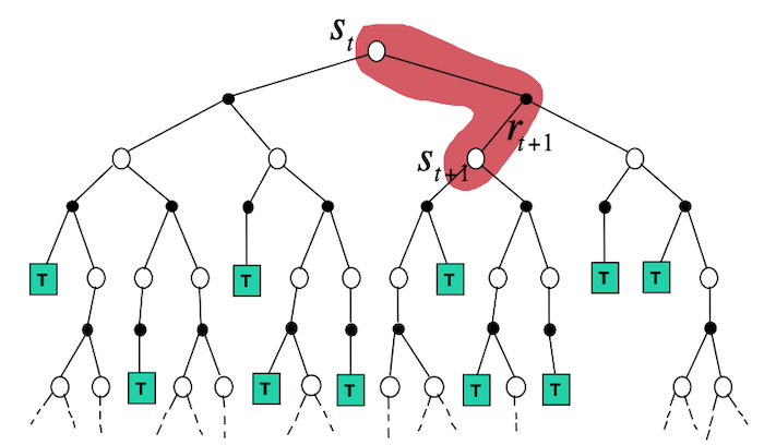
The fundamental idea of temporal-difference (TD) learning is to remove the need of waiting until the end of an episode to get $G_t$ in MC methods, by taking a single step and update using $R_{t+1} + \gamma V(S_{t+1}) \approx G_t$. Note that when the estimates are correct, i.e. $V(S_{t+1}) = v_\pi(S_{t+1})$, then $\mathbb{E}[R_{t+1} + \gamma V(S_{t+1})] = \mathbb{E}[G_t]$.
As we have seen, incremental MC methods for evaluating $V$, can be written as $V_{k+1}(S_t) = V_{k}(S_t) + \alpha \left( G_t - V_{k}(S_t) \right)$. Using bootstrapping, this becomes:
\[V_{k+1}(S_t) = V_{k}(S_t) + \alpha \left( R_{t+1} + \gamma V_k(S_{t+1}) - V_{k}(S_t) \right)\]This important update is called $\textbf{TD(0)}$, as it is a specific case of TD(lambda). The error term that is used to update our estimate, is very important in RL and Neuroscience. It is called the TD Error:
\[\delta_t := R_{t+1} + \gamma V(S_{t+1}) - V(S_t)\]Importantly $\text{TD}(0)$ always converges to $v_\pi$ if $\alpha$ decreases according to the usual stochastic conditions (e.g. $\alpha = \frac{1}{t}$). Although, the theoretical difference in speed of convergence of TD(0) and MC methods is still open, the former often converges faster in practice.
![]() Side Notes:
Side Notes:
- $\delta_t$ is the error in $V(S_t)$ but is only available at time $t+1$.
- The MC error can be written as a sum of TD errors if $V$ is not updated during the episode: $G_t - V(S_t) = \sum_{k=t}^{T-1} \gamma^{k-t} \delta_k$
- Updating the value with the TD error, is called the backup
- the name comes from the fact that you look at the difference between estimates of consecutive time.
- For batch updating (i.e. single batch of data that is processed multiple times and the model is updated after each batch pass), MC and TD(0) do not in general find the same answer. MC methods find the estimate that minimizes the mean-squared error on the training set, while TD(0) finds the maximum likelihood estimate of the Markov Process. For example, suppose we have 2 states $A$, $B$ and a training data $\{(A:0:B:0), (B:1), (B:1), (B:0)\}$. What should $V(A)$ be? There are at least 2 answers that make sense. MC methods would answer $V(A)=0$ because every time $A$ has been seen, it resulted in a reward of $0$. This doesn't take into account the Markov property. Conversely, $TD(0)$ would answer $V(A)=0.5$ because $100\%$ of $A$ transited to $B$. Using the Markov assumption, the rewards should be independent of the past once we are in state $B$. I.e. $V(A)=V(B)=\frac{2}{4}=\frac{1}{2}$.
On-Policy TD GPI (SARSA)
Similarly to MC methods, we need an action-value function $q_\pi$ instead of a state one $v_\pi$ because we do not know the dynamics and thus cannot simply learn the policy from $v_\pi$. Replacing TD estimates in on policy MC GPI, we have:
- Generalized Policy Evaluation (Prediction): this update is done for every transition from a non-terminal state $S_t$ (set $Q(s_{terminal},A_{t+1})=0$):
- Policy Improvement: make a GLIE policy $\pi$ from $Q$. Note that the policy improvement theorem still holds.
![]() Side Notes:
Side Notes:
- The update rule uses the values $(S_t, A_t, R_{t+1}, S_{t+1}, A_{t+1})$, which gave its name.
- As with On policy MC GPI, you have to ensure sufficient exploration which can be done using an $\epsilon\text{-greedy}$ policy.
- As with MC, the algorithm converges to an optimal policy as long as the policy is GLIE.
In python pseudo-code:
def sarsa(game, states, actions, n=..., eps=..., gamma=..., alpha=...):
    """SARSA using epsilon greedy policy."""
    Q = defaultdict(lambda x: 0)
    pi = q_to_eps_pi(Q, eps, actions, states) # defined in on policy MC
    for _ in range(n):
        s_t = game() #initializes the state
        a_t = sample(pi, s_t)
        while s_t not is terminal:
            s_t1, r_t = game(s_t, a_t) # single run
            # compute A_{t+1} for update
            a_t1 = sample(pi, s_t1)
            Q[(s_t, a_t)] += alpha * (r_t + gamma*Q[(s_t1, a_t1)] - Q[(s_t, a_t)])
            pi = update_eps_policy(Q, pi, s_t, actions, eps) # defined in on policy MC
            s_t, a_t = s_t1, a_t1
    return pi
Off Policy TD GPI (Q-Learning)
Just as with off-policy MC, TD can be written as an off-policy algorithm. In this case, the TD error is not computed with respect to the next sample but with respect to the current optimal greedy policy (i.e. the one maximizing the current action-value function $Q$)
- Generalized Policy Evaluation (Prediction):
- Policy Improvement: make a GLIE policy $\pi$ from $Q$.
The algorithm can be proved to converge as long as all state-action pairs continue being updated.
In python pseudo-code:
def q_learning(game, states, actions, n=..., eps=..., gamma=..., alpha=...):
    """Q learning."""
    Q = defaultdict(lambda x: 0)
    pi = q_to_eps_pi(Q, eps, actions, states) # defined in on policy MC
    for _ in range(n):
        s_t = game() # initializes the state
        while s_t not is terminal:
            a_t = sample(pi, s_t)
            s_t1, r_t = game(s_t, a_t) # single run
            a_best = argmax(Q[(s_t1, a)] for a in actions)
            Q[(s_t, a_t)] += alpha * (r_t + gamma*a_best - Q[(s_t, a_t)])
            pi = update_eps_policy(Q, pi, s_t, actions, eps) # defined in on policy MC
            s_t, = s_t1
    return pi