Linear programming
Linear programming (LP) deals with linear objective functions subject to linear constraints (equality and inequality). Any LP problem can be expressed in a canonical form:
\[\begin{array}{cc} \max_x & f(x)=\mathbf{c}^T\mathbf{x} \\ \text{s.t.} & A\mathbf{x} \leq \mathbf{b} \\ & \mathbf{x} \geq \mathbf{0} \end{array}\]The constraints $A\mathbf{x} \leq b$ are called the main constraints, while $\mathbf{x} \geq \mathbf{0}$ are the non-negativity constraints. The set of points that satisfy all constraints form the feasible region. This region is a convex polytope (points between in a polyhedron that is defined by intersecting lines. Formally, it is the intersection of a finite number of half-spaces) defined by the linear inequalities. The goal is to find the point in the polyhedron associated with the maximum (or minimum) of the function. Note: for unbounded problems (i.e. objective function can take large values) the feasible region is infinite.
Let's look at the simple example used in this blog, from whom I borrowed the nice plots:
\[\begin{array}{cc} \max_x & f(\mathbf{x})=3x_1+2x_2 \\ \text{s.t.} & 2x_1 + x_2 \leq 100 \\ & x_1 + x_2 \leq 80 \\ & x_1 \leq 40 \\ & x_1, x_2 \geq 0 \\ \end{array}\]The feasible region in this case is :

We now have to find the point in this region which maximizes $3x_1+2x_2$. For any given $z$ let's consider the set of all points whose cost is $\mathbf{c}^T\mathbf{x}=z$ (level curves of the objective function). This is the line described by $z=3x_1+2x_2$. Note that $\forall z$ these lines are parallel to each other and perpendicular to $\mathbf{c}=(3,2)$. In particular, increasing $z$ corresponds to moving the line $z=3x_1+2x_2$ along the direction of $\mathbf{c}$ ($\nabla f(\mathbf{x})=\mathbf{c}$):
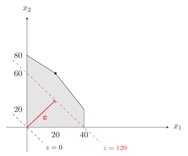
As we want to maximize $z$, we would like to move the line as much as possible along $\mathbf{c}$, while staying in the feasible region. The best we can do is $z=180$, and the vector $\mathbf{x}=(20,60)$ is the corresponding optimal solution:

Note that the optimal solution $\mathbf{x}=(20,60)$ is a vertex of the polytope. We will show later that this is always the case.
Canonical and Slack form
![]() Side Notes: Beware that the term standard form is very often used in the literature to mean different things. For example in Bertismas and Tsitsiklis the standard form is equivalent to the canonical form we have seen above, while the standard form in Vanderbei' book refers to what I will call the slack form. I thus decided not to use the term "standard form".
Side Notes: Beware that the term standard form is very often used in the literature to mean different things. For example in Bertismas and Tsitsiklis the standard form is equivalent to the canonical form we have seen above, while the standard form in Vanderbei' book refers to what I will call the slack form. I thus decided not to use the term "standard form".
Canonical Form:
\[\begin{array}{cc} \max_x & f(x)=\mathbf{c}^T\mathbf{x} \\ \text{s.t.} & A\mathbf{x} \leq \mathbf{b} \\ & \mathbf{x} \geq \mathbf{0} \end{array}\]Slack Form:
\[\begin{array}{cc} \min_x & f(x)=\mathbf{c}^T\mathbf{x} \\ \text{s.t.} & A\mathbf{x} = \mathbf{b} \\ & \mathbf{x} \geq \mathbf{0} \end{array}\]The canonical form is very natural and thus often used to develop the theory, but the slack form is usually the starting points for all algorithms as it is computationally more convenient.
Any general LP problem can be converted back and forth to these 2 forms. Let's first see how to convert general LP problems to the canonical form:
- Convert to maximizing problems, by multiplying the objective function of minimizing problems by $-1$.
- Convert constraints to $\leq$: $\forall i$ such that there exist a main constraint of the form $\mathbf{a}_i^T \mathbf{x} \geq b_i$, change it to $(-\mathbf{a}_i)^T\mathbf{x}\leq (-b_i)$.
- Remove equality constraints $\sum_j a_{ij}^T x_j = b_i$ by solving for a $x_j$ associated with a non zero $a_{ij}$ and substituting this $x_j$ whenever it appears in the objective function or constraints. This removes one constraint and one variable from the problem.
- Restrict variables to be non-negative by replacing unrestricted or negative $x_j$ by $x_j=x_j^{+}-x_j^{-}$ where $x_j^{+}, x_j^{-} \geq 0$ . Indeed, any real number can be written as the difference between 2 non-negative numbers.
Let's now see how to convert general LP problems to the slack form:
- Convert to minimizing problems, by multiplying the objective function of maximizing problems by $-1$.
- Restrict variables to be non-negative by replacing unrestricted or negative $x_j$ by $x_j=x_j^{+}-x_j^{-}$ where $x_j^{+}, x_j^{-} \geq 0$.
- Eliminate inequality constraints $\mathbf{a}_i^T\mathbf{x}\leq b_i$ by introducing a slack variable : $\mathbf{a}_i^T\mathbf{x} + s_i = b_i$, $s_i \geq 0$. Similarly for $\mathbf{a}_i^T\mathbf{x} \geq b_i$, introduce a surplus variable $\mathbf{a}_i^T\mathbf{x} - s_i = b_i$, $s_i \geq 0$.
![]() Side Notes:
Side Notes:
- when converting from the canonical form to the slack one, the objective function $f(x)=\mathbf{c}^T\mathbf{x}$ is unmodified because $\mathbf{x}^{slack}=[\mathbf{x}^{canonical}; \mathbf{s}]$ and $\mathbf{c}^{slack}=[\mathbf{c}^{canonical}; \mathbf{0}]$, and the constraints are simply a re-parametrization using slack variables.
- In the slack form, $A \in \mathbb{R}^{m \times n}$ has full row rank $m$ (i.e. $n > m$), otherwise there would be "no room for optimization" as there would be a single or no solution
We have already seen an example which visualized the canonical form of the problem. I.e. for $\mathbf{x} \in \mathbb{R}^{n'}$ the feasible set is a polytope with at most $m'$ vertices (described by $A \mathbf{x} \geq \mathbf{b}$) in a $n'$ dimensional space.
In the slack form with $m$ constraints and $\mathbf{x} \in \mathbb{R}^{n}$, the constraints force $\mathbf{x}$ to lie on an $(n-m)$ dimensional subspace (each constraint removes a degree of freedom of $\mathbf{x}$). Once in that $(n-m)$ dimensional subspace, the feasible set is only bounded by the non-negativity constraints $\mathbf{x} \geq \mathbf{0}$. I.e. the slack form of the problem, can be seen as minimizing a function in a polytope in a $(n-m)$ dimensional subspace. Importantly, the polytope has the exact same shape as for the canonical form, but lives is a different space!
Duality
In optimization, it is very common to convert constrained problems to a relaxed unconstrained formulation, by allowing constraints to be violated but adding "a price" $\mathbf{y}$ to pay for that violation. When the price is correctly chosen, the solution of both problems becomes the same (by letting $\mathbf{y} \to \infty$ you effectively don't allow any violation of the constraints:). This is the key idea behind the well known Lagrange Multipliers. Let's call the problem formulation we have seen until know the primal problem. Then the slack form of the primal problem can be relaxed as:
\[\begin{array}{cc} \min_x & \mathbf{c}^T\mathbf{x} + \mathbf{y}^T (\mathbf{b}-A\mathbf{x}) \\ \text{s.t.} & \mathbf{x} \geq \mathbf{0} \end{array}\]Let $g(\mathbf{y})$ be the optimal cost of the relaxed problem as a function of the violation price $\mathbf{y}$. $g(\mathbf{y})$ is a lower bound to the the optimal solution $\mathbf{x}^{*}$ of the constraint problem (weak duality theorem). Indeed ($A\mathbf{x}^*=\mathbf{b}$):
\[g(\mathbf{y})=min_{\mathbf{x} \geq \mathbf{0}} \left( \mathbf{c}^T\mathbf{x} + \mathbf{y}^T (\mathbf{b}-A\mathbf{x}) \right) \leq \mathbf{c}^T\mathbf{x}^* + \mathbf{y}^T (\mathbf{b}-A\mathbf{x}^*) = \mathbf{c}^T\mathbf{x}^*\]The goal is thus to find the tightest lower bound $\max_y g(\mathbf{y})$, and is called the dual problem. The problem can be simplified by noting that:
\[\begin{aligned} \max_\mathbf{y} g(\mathbf{y}) &= \max_\mathbf{y} & min_{\mathbf{x} \geq \mathbf{0}} \left( \mathbf{c}^T\mathbf{x} + \mathbf{y}^T (\mathbf{b}-A\mathbf{x}) \right) \\ &= \max_\mathbf{y} & \mathbf{y}^T \mathbf{b} + min_{\mathbf{x} \geq \mathbf{0}} \left( (\mathbf{c}^T - \mathbf{y}^T A)\mathbf{x} \right)\\ &= \max_\mathbf{y} & \mathbf{y}^T \mathbf{b} + 0 \\ &\ \ \ \text{ s.t.} & \mathbf{y}^TA \leq \mathbf{c}^T \end{aligned}\]Where the last line comes from the fact that $min_{\mathbf{x} \geq \mathbf{0}} \left( (\mathbf{c}^T + \mathbf{y}^T A)\mathbf{x} \right)$ is $0$ if $\mathbf{y}^TA \leq \mathbf{c}^T$ and $-\infty$ otherwise.
The dual problem is thus another LP problem that can be written as:
\[\begin{array}{cc} \max_y & \mathbf{y}^T \mathbf{b} \\ \text{s.t.} & A^T\mathbf{y} \leq \mathbf{c} \end{array}\]![]() Side Notes:
Side Notes:
- Each main constraint in the primal LP, becomes a variable in the dual LP. Similarly, each variable in the primal LP becomes a main constraint in the dual LP. The objective is reversed.
- The dual of the dual is the primal.
- Weak Duality Theorem: if $\mathbf{x}$ is a feasible solution to the primal LP and $\mathbf{y}$ is a feasible solution of the dual LP, then $\mathbf{y}^T\mathbf{b} \leq \mathbf{c}^T\mathbf{x}$.
- Strong Duality Theorem: if one of the dual / primal LP has a solution, so does the second one, and the respective objective function are equal.
- Complementary Slackness $\mathbf{x}, \ \mathbf{p}$ are optimal solutions for the primal and dual LP respectively iff $y_i(\mathbf{a}_i^T\mathbf{x}-b_i)=0, \ \forall i$ and $x_j(c_j-\mathbf{p}^T\mathbf{a}_j)=0, \forall j$. I.e. for the primal LP, either the constraints are tight or the corresponding dual variable $p_j$ is 0 (and vis-versa).
- Importantly the dual problem is also a LP, meaning that the dual feasible set is a convex polytope. The polytope is now defined by $n$ constraints and lives in a $m$ dimensional space instead of the reverse in the primal case ($m$ constraints, $n$ dimensional space).
- In case the primal LP is in the canonical form, the dual LP can be written as :
Canonical Primal LP:
\[\begin{array}{cc} \max_x & \mathbf{c}^T\mathbf{x} \\ \text{s.t.} & A\mathbf{x} \leq b \\ & \mathbf{x} \geq \mathbf{0} \end{array}\]Associated Dual LP:
\[\begin{array}{cc} \min_y & \mathbf{b}^T\mathbf{y} \\ \text{s.t.} & A^T\mathbf{y} \geq \mathbf{c} \\ & \mathbf{y} \geq \mathbf{0} \end{array}\]![]() Resources: the intuitive link between the primal and dual form explained above comes from the very good Introduction to Linear Optimization. Another great resource is the coursera course on discrete optimization (lecture LP6 week 5).
Resources: the intuitive link between the primal and dual form explained above comes from the very good Introduction to Linear Optimization. Another great resource is the coursera course on discrete optimization (lecture LP6 week 5).