Curse of dimensionality
The Curse of dimensionality refers to various practical issues when working with high dimensional data. These are often computational problems or counter intuitive phenomenas, coming from our Euclidean view of the 3 dimensional world.
They are all closely related but I like to think of 3 major issues with high dimensional inputs $x \in \mathbb{R}^d, \ d \ggg 1$:
Sparsity Issue
You need exponentially more data to fill in a high dimensional space. I.e. if the dataset size is constant, increasing the dimensions makes your data sparser.
![]() Intuition : The volume size grows exponentially with the number of dimensions. Think of filling a $d$ dimensional unit hypercube with points at a $0.1$ interval. In 1 dimension we need $10$ of these points. In 2 dimension we already need 100 of these. In $d$ dimension we need $10^d$ observation !
Intuition : The volume size grows exponentially with the number of dimensions. Think of filling a $d$ dimensional unit hypercube with points at a $0.1$ interval. In 1 dimension we need $10$ of these points. In 2 dimension we already need 100 of these. In $d$ dimension we need $10^d$ observation !
Let's look at a simple example :
Imagine we trained a certain classifier for distinguishing between ![]() and
and ![]() . Now we want to predict the class of an unkown observation
. Now we want to predict the class of an unkown observation ![]() . Let's assume that:
. Let's assume that:
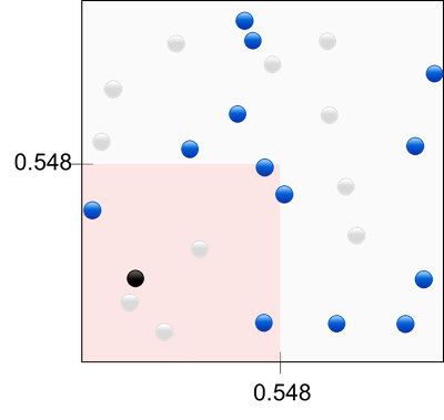
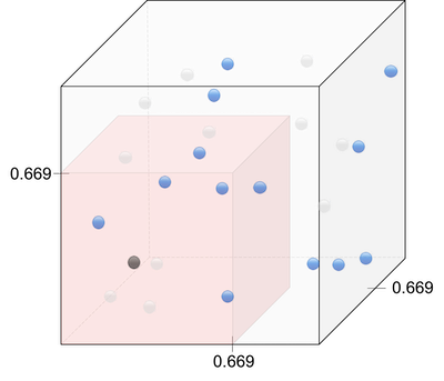
- All features are given in percentages $[0,1]$
- The algorithm is non-parametric and has to look at the points in the surrounding hypercube, which spans $30\%$ of the input space (see below).
Given only 1 feature (1D), we would simply need to look at $30\%$ of the dimension values. In 2D we would need to look at $\sqrt{0.3}=54.8\%$ of each dimensions. In 3D we would need $\sqrt[3]{0.3}=66.9\%$ of in each dimensions. Visually:

In order to keep a constant support (i.e. amount of knowledge of the space), we thus need more data when adding dimensions. In other words, if we add dimensions without adding data, there will be large unknown sub-spaces. This is called sparsity.
I have kept the same number of observation in the plots, so that you can appreciate how "holes" appear in our training data as the dimension grows.
![]() Disadvantage : The data sparsity issue causes machine learning algorithms to fail finding patterns or to overfit.
Disadvantage : The data sparsity issue causes machine learning algorithms to fail finding patterns or to overfit.
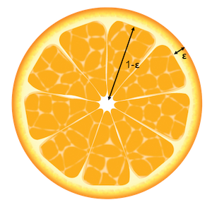
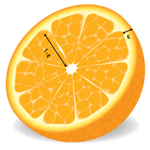
Points are further from the center
Basically, the volume of a high dimensional orange is mostly in its skin and not in the pulp! Which means expensive high dimensional juices ![]()
![]()
![]() Intuition : The volume of a sphere depends on $r^d$. The skin has a slightly greater $r$ than the pulp, in high dimensions this slight difference will become very important.
Intuition : The volume of a sphere depends on $r^d$. The skin has a slightly greater $r$ than the pulp, in high dimensions this slight difference will become very important.
If you're not convinced, stick with my simple proof. Let's consider a $d$ dimensional unit orange (i.e. $r=1$), with a skin of width $\epsilon$. Let's compute the ratio of the volume in the skin to the total volume of the orange. We can avoid any integrals by noting that the volume of a hypersphere is proportional to $r^d$ i.e. : $V_{d}(r) = k r^{d}$.
\[\begin{align*} ratio_{skin/orange}(d) &= \frac{V_{skin}}{V_{orange}} \\ &= \frac{V_{orange} - V_{pulp}}{V_{orange}} \\ &= \frac{V_{d}(1) - V_{d}(1-\epsilon) }{V_{d}(1)} \\ &= \frac{k 1^d - k (1-\epsilon)^d}{k 1^d} \\ &= 1 - (1-\epsilon)^d \end{align*}\]Taking $\epsilon = 0.05$ as an example, here is the $ratio_{skin/orange}(d)$ we would get:


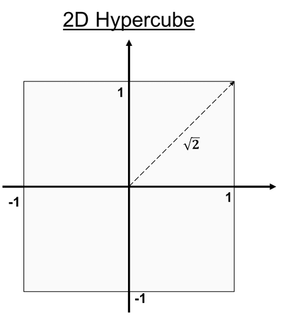
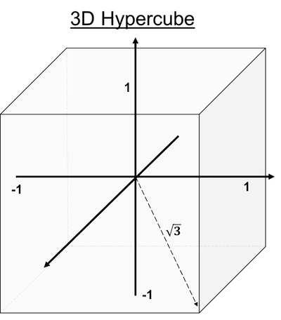
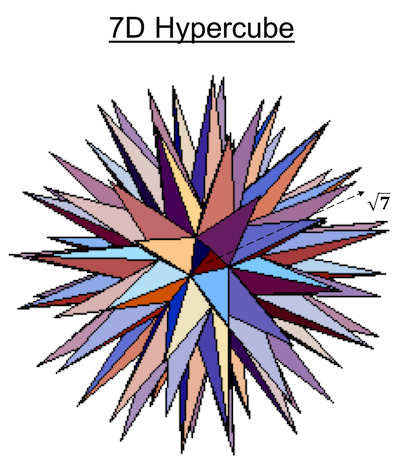
![]() Side Notes : The same goes for hyper-cubes: most of the mass is concentrated at the furthest points from the center (i.e. the corners). That's why you will sometimes hear that hyper-cubes are "spiky". Think of the $[-1,1]^d$ hyper-cube: the distance from the center of the faces to the origin will trivially be $1 \ \forall d$, while the distance to each corners will be $\sqrt{d}$ (Pythagorean theorem). So the distance to corners increases with $d$ but not the center of the faces, which makes us think of spikes. This is why you will sometimes see such pictures:
Side Notes : The same goes for hyper-cubes: most of the mass is concentrated at the furthest points from the center (i.e. the corners). That's why you will sometimes hear that hyper-cubes are "spiky". Think of the $[-1,1]^d$ hyper-cube: the distance from the center of the faces to the origin will trivially be $1 \ \forall d$, while the distance to each corners will be $\sqrt{d}$ (Pythagorean theorem). So the distance to corners increases with $d$ but not the center of the faces, which makes us think of spikes. This is why you will sometimes see such pictures:
Euclidean distance becomes meaningless
There's nothing that makes Euclidean distance intrinsically meaningless for high dimensions. But due to our finite number of data, 2 points in high dimensions seem to be more "similar" due to sparsity and basic probabilities.
![]() Intuition :
Intuition :
- Let's consider the distance between 2 points $\mathbf{q}$ and $p$ that are close in $\mathbb{R}^d$. By adding independent dimensions, the probability that these 2 points differ greatly in at least one dimension grows (due to randomness). This is what causes the sparsity issue. Similarly, the probability that 2 points far away in $\mathbb{R}$ will have at least one similar dimension in $\mathbb{R}^d, \ d'>d$, also grows. So basically, adding dimensions makes points seem more random, and the distances thus become less useful.
- Euclidean distance accentuates the point above. Indeed, by adding dimensions, the probability that $\mathbf{x}^{(1)}$ and $\mathbf{x}^{(2)}$ points have at least one completely different feature grows. i.e. $\max_j \, (x_j^{(1)}, x_j^{(2)})$ increases. The Euclidean distance between 2 points is $D(\mathbf{x}^{(1)},\mathbf{x}^{(2)})=\sqrt{\sum_{j=1}^D (\mathbf{x}_j^{(1)}-\mathbf{x}_j^{(2)})^2}$. Because of the squared term, the distance depends strongly on $max_j \, (x_j^{(1)}-x_j^{(2)})$. This results in less relative difference between distances of "similar" and "dissimilar points" in high dimensions. Manhattan ($L_1$) or fractional distance metrics ($L_c$ with $c<1$) are thus preferred in high dimensions.
In such discussions, people often cite a theorem stating that for i.i.d points in high dimension, a query point $\mathbf{x}^{(q)}$ converges to the same distance to all other points $P=\{\mathbf{x}^{(n)}\}_{n=1}^N$ :
\[\lim_{d \to \infty} \mathop{\mathbb{E}} \left[\frac{\max_{n} \, (\mathbf{x}^{(q)},\mathbf{x}^{(n)})}{\min_{n} \, (\mathbf{x}^{(q)},\mathbf{x}^{(n)})} \right] \to 1\]![]() Practical : using dimensionality reduction often gives you better results for subsequent steps due to this curse. It makes the algorithm converge faster and reduces overfitting. But be careful not to underfit by using too few features.
Practical : using dimensionality reduction often gives you better results for subsequent steps due to this curse. It makes the algorithm converge faster and reduces overfitting. But be careful not to underfit by using too few features.
![]() Side Notes :
Side Notes :
- Although the curse of dimensionality is a big issue, we can find effective techniques in high-dimensions because:
- Real data is often confined to a lower effective dimensionality (e.g. a low dimensional manifold in a higher dimensional space).
- Interpolation-like techniques can overcome some of the sparsity issues due to the local smoothness of real data.
- You often see plots of the unit $d$-ball volume vs its dimensionality. Although the non-monotonicity of such plots is intriguing, they can erroneously make you believe that high dimensional hypersphere are smaller than low dimensional ones. This does not make sense as a lower dimensional hypersphere can always be fitted in a higher dimensional one. The issue arises from comparing apple and oranges (no puns intended
 ) due to different units: Is $0.99 m^2$ really smaller than $1 m$?
![]() Resources : Great post about the curse of dimensionality in classification which inspired me, On the Surprising Behavior of Distance Metrics in High Dimensional Space is a famous paper which proposes the use of fractional distance metrics, nice blog of simulations.
Resources : Great post about the curse of dimensionality in classification which inspired me, On the Surprising Behavior of Distance Metrics in High Dimensional Space is a famous paper which proposes the use of fractional distance metrics, nice blog of simulations.