Reinforcement learning
In Reinforcement Learning (RL), the sequential decision-making algorithm (an agent) interacts with an environment it is uncertain about. The agent learns to map situations to actions to maximize a long term reward. During training, the action it chooses are evaluated rather than instructed.
![]() Example: Games can very naturally be framed in a RL framework. For example, when playing tennis you are not told how good every movement you make is, but you are given a certain reward if you win the whole game.
Example: Games can very naturally be framed in a RL framework. For example, when playing tennis you are not told how good every movement you make is, but you are given a certain reward if you win the whole game.
![]() Side Notes: Games could also be framed in a supervised problem. The training set would consist in many different states of the environment and the optimal action to take in each of those. Creating such a dataset is not possible for most applications as it requires to enumerate the exponential number of states and to know the associated best action (e.g. exact rotation of all your joints when you play tennis). Note that during supervised training, the feedback indicates the correct action independently to the chosen action. The RL framework is a lot more natural as the agent is trained by playing the game. Importantly, the agent interacts with the environment such that the states that it will visit depend on previous actions. So it is a chicken-egg problem where it will unlikely reach good states before being trained, but it has to reach good states to get reward and train effectively. This leads to training curves that start with very long plateaus of low reward until it reaches a good state (somewhat by chance) and then learn quickly. In contrast, supervised methods have very steep loss curves at the start.
Side Notes: Games could also be framed in a supervised problem. The training set would consist in many different states of the environment and the optimal action to take in each of those. Creating such a dataset is not possible for most applications as it requires to enumerate the exponential number of states and to know the associated best action (e.g. exact rotation of all your joints when you play tennis). Note that during supervised training, the feedback indicates the correct action independently to the chosen action. The RL framework is a lot more natural as the agent is trained by playing the game. Importantly, the agent interacts with the environment such that the states that it will visit depend on previous actions. So it is a chicken-egg problem where it will unlikely reach good states before being trained, but it has to reach good states to get reward and train effectively. This leads to training curves that start with very long plateaus of low reward until it reaches a good state (somewhat by chance) and then learn quickly. In contrast, supervised methods have very steep loss curves at the start.
![]() Resources : The link and differences between supervised and RL is described in details by A. Barto and T. Dietterich.
Resources : The link and differences between supervised and RL is described in details by A. Barto and T. Dietterich.
In RL, future states depend on current actions, thus requiring to model indirect consequences of actions and planning. Furthermore, the agent often has to take actions in real-time while planning for the future. All of the above makes it very similar to how humans learn, and is thus widely used in psychology and neuroscience.
![]() Resources : All this section on RL is highly influenced by Sutton and Barto's introductory book.
Resources : All this section on RL is highly influenced by Sutton and Barto's introductory book.
Exploration vs Exploitation
A fundamental trade-off in RL is how to balance exploration and exploitation. Indeed, we often assume that the agent has to maximize its reward over all episodes. As it often lacks knowledge about the environment, it has to decide between taking the action it currently thinks is the best, and taking new actions to learn about how good these are (which might bring higher return in the long run).
![]() Example: Lets consider a simplified version of RL - Multi-armed Bandits - to illustrate this concept (example and plots from Sutton and Barto):
Example: Lets consider a simplified version of RL - Multi-armed Bandits - to illustrate this concept (example and plots from Sutton and Barto):
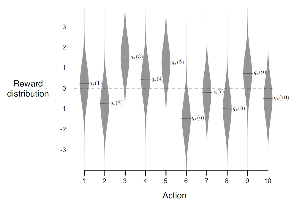
Let's assume that you go in a very generous casino. I.e. an utopic casino in which you can make money in the long run (spoiler alert: this doesn't exist, and in real-life casinos the best action is always to leave ![]() ). This casino contains 10-slot machines, each of these give a certain reward $r$ when the agent decides to play on them. The agent can stay the whole day in this casino and wants to maximize its profit.
). This casino contains 10-slot machines, each of these give a certain reward $r$ when the agent decides to play on them. The agent can stay the whole day in this casino and wants to maximize its profit.
Although the agent doesn't know it, the rewards are sampled as $r \sim \mathcal{N}(\mu_a, 1)$, and each of the 10 machines have a fixed $\mu_a$ which were sampled from $\mathcal{N}(0, 1)$ when building the casino. The actual reward distributions are the following (where $q_{*}(a)$ denote the expected return when choosing slot $a$):
A good agent would try to estimate $Q_t(a) = q_{*}(a)$, where the subscript $t$ indicates that the estimate depends on the time (the more the agent plays the better the estimates should be). The most natural estimate $Q_t(a)$ is to average over all rewards when taking action $a$. At every time step $t$ there's at least one action $\hat{a}=\arg\max_a Q_t(a)$ which the agent believes maximizes $q_{*}(a)$. Taking the greedy action $\hat{a}$ exploits your current beliefs of the environment. This might not always be the "best action", indeed if $\hat{a} \neq a^{*}$ then the agents estimates of the environment are wrong and it would be Better to take a non greedy action $a \neq \hat{a}$ and learn about the environment (supposing it will still play many times). Such actions explore the environment to improve estimates.
During exploration, the reward is often lower in the short run, but higher in the long run because once you discovered better actions you can exploit them many times. Whether to explore or exploit is a complex problem that depends on your current estimates, uncertainties, and the number of remaining steps.
Here are a few possible exploration mechanisms:
- $\pmb{\epsilon}\mathbf{-greedy}$: take the greedy action with probability $1-(\epsilon-\frac{\epsilon}{10})$ and all other actions with probability $\frac{\epsilon}{10}$.
- *Upper-Confidence Bound ** (UCB): $\epsilon\text{-greedy}$ forces the non greedy actions to be tried uniformly. It seems natural to prefer actions that are nearly greedy or particularly uncertain. This can be done by adding a term that measures the variance of the estimate of $Q_t(a)$. Such a term should be inversely proportional to the number of times we have seen an action $N_t(a)$. We use $\frac{\log t}{N_t(a)}$ in order to force the model to take an action $a$ if it has not been taken in a long time (i.e.* if $t$ increases but not $N_t(a)$ then $\frac{\log t}{N_t(a)}$ increases). The logarithm is used in order have less exploration over time but still an infinite amount:
Optimistic Initial Values: gives a highly optimistic $Q_1(a), \ \forall a$ (e.g. $Q_1(a)=5$ in our example, which is a lot larger than $q_{*}(a)$). This ensures that all actions will be at least sampled a few times before following the greedy policy. Note that this permanently biases the action-value estimates when estimating $Q_t(a)$ through averages (although the biases decreases).
Gradient Bandit Algorithms: An other natural way of choosing the best action would be to keep a numerical preference for each action $H_t(a)$. And sample more often actions with larger preference. I.e. sample from $\pi_t := \text{softmax}(H_t)$, where $\pi_t(a)$ denotes the probability of taking action $a$ at time $t$. The preference can then be learned via stochastic gradient ascent, by increasing $H_t(A_t)$ if the reward due to the current action $A_t$ is larger than the current average reward $\bar{R}_t$ (decreasing $H_t(A_t)$ if not). The non selected actions $a \neq A_t$ are moved in the opposite direction. Formally:
By running all the different strategies for different hyperparameters and averaging over 1000 decisions, we get:
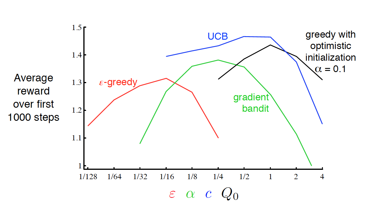
We see that UCB performs best in this case, and is the most robust with regards to its hyper-parameter $c$. Although UCB tends to work well, this will not always be the case (No Free Lunch Theorem again).
![]() Side Notes:
Side Notes:
- In non-stationary environments (I.e. the reward probabilities are changing over time), it is important to always explore as the optimal action might change over time. In such environment, it is better to use exponentially decaying weighted average for $Q_t(a)$. I.e. give more importance to later samples.
- The multi-armed bandits problem, is a simplification of RL as future states and actions are independent of the current action.
- We will see other ways of maintaining exploration in future sections.
Markov Decision Process
Markov Decision Processes (MDPs) are a mathematical idealized form of the RL problem that suppose that states follow the Markov Property. I.e. that future states are conditionally independent of past ones given the present state: $S_{t+1} \perp \{S_{i}\}_{i=1}^{t-1} \vert S_t$.
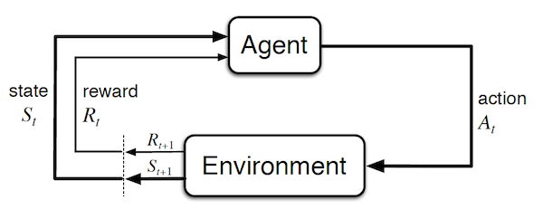
Before diving into the details, it is useful to visualize how simple a MDP is (image taken from Sutton and Barto):
Important concepts:
- Agent: learner and decision maker. This corresponds to the controller in classical control theory.
- Environment: everything outside of the agent. I.e. what it interacts with. It corresponds to the plant in classical control theory. Note that in the case of a human / robot, the body should be considered as the environment rather than as the agent because it cannot be modified arbitrarily (the boundary is defined by the lack of possible control rather than lack of knowledge).
- Time step t: discrete time at which the agent and environment interact. Note that it doesn't have to correspond to fix real-time intervals. Furthermore, it can be extended to the continuous setting.
- State $S_t = s \in \mathcal{S}$ : information available to the agent about the environment.
- Action $A_t=a \in \mathcal{A}$ : action that the agent decides to take. It corresponds to the control signal in classical control theory.
- Reward $R_{t+1} = r \in \mathcal{R} \subset \mathbb{R}$: a value which is returned at each step by a (deterministic or stochastic) reward signal function depending on the previous $S_t$ and $A_t$. Intuitively, the reward corresponds to current (short term) pain / pleasure that the agent is feeling. Although the reward is computed inside the agent / brain, we consider them to be external (given by the environment) as they cannot be modified arbitrarily by the agent. The reward signal we choose should truly represent what we want to accomplish , not how to accomplish it (such prior knowledge can be added in the initial policy or value function). For example, in chess, the agent should only be rewarded if it actually wins the game. Giving a reward for achieving subgoals (e.g. taking out an opponent's piece) could result in reward hacking (i.e. the agent might found a way to achieve large rewards without winning).
- Return $G_t := \sum_{\tau=1}^{T-t} \gamma^{\tau-1} R_{t+\tau} \text{, with } \gamma \in [0,1[$: the expected discounted cumulative reward, which has to be maximized by the agent. Note that the discounting factor $\gamma$, has a two-fold use. First and foremost, it enables to have a finite $G_t$ even for continuing tasks $T=\infty$ (opposite of episodic tasks) assuming that $R_t$ is bounded $\forall t$. It also enables to encode the preference for rewards in the near future, and is a parameter that can be tuned to select the "far-sightedness" of your agent ("myopic" agent with $\gamma=0$, "far-sighted" as $\gamma \to 1$). Importantly, the return can be defined in a recursive manner :
- The dynamics of the MDP: $p(s', r\vert s, a) := P(S_{t+1}=s', R_{t+1}=r \vert S_t=s, A_t=a)$. In a MDP, this probability completely characterizes the network dynamics due to the Markov property. Some useful functions that can be derived from it are:
- State-transition probabilities
- Expected rewards for state-actions pairs:
- Expected rewards for state-actions-next state triplets:
- Policy $\pi(a\vert s)$: a mapping from states to probabilities over actions. Intuitively, it corresponds to a "behavioral function". Often called stimulus-response in psychology.
- State-value function for policy $\pi$, $v_\pi(s)$: expected return for an agent that follows a policy $\pi$ and starts in state $s$. Intuitively, it corresponds to how good it is to be in a certain state $s$ (long term). This function is not given by the environment but is often predicted by the agent. Similar to the return, the value function can also be defined recursively, by the very important Bellman equation :
- Action-value function (Q function) for policy $\pi$, $q_\pi(s,a)$: expected total reward and agent can get starting from a state $s$. Intuitively, it corresponds to how good it is to be in a certain state $s$ and take specific action $a$ (long term). A Bellman equation can be derived in a similar way to the value function:
- Model of the environment: an internal model in the agent to predict the dynamic of the environment (e.g. probability of getting a certain reward or getting in a certain state for each action). This is only used by some RL agents for planning.
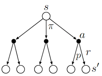
To schematically represents what different algorithms do, it is useful to look at Backup Diagrams. These are trees that are constructed by unrolling all the possible actions and states. White nodes represent a state, from which the agent will follow its policy to select one possible action (black node). The environment will then sample through the dynamics to bring the agent to a new state. Green nodes will be used to denote terminal nodes, and the path taken by the algorithm will be shown in red. Unlike transition graphs, state nodes are not unique (e.g. states can be their own successors). Example:
![]() Side Notes : We usually assume that we have a finite MDP. I.e. that $\mathcal{R},\mathcal{A},\mathcal{S}$ are finite. Dealing with continuous state and actions pairs requires approximations. One possible way of converting a continuous problem to a finite one, is to discretized the state and actions space.
Side Notes : We usually assume that we have a finite MDP. I.e. that $\mathcal{R},\mathcal{A},\mathcal{S}$ are finite. Dealing with continuous state and actions pairs requires approximations. One possible way of converting a continuous problem to a finite one, is to discretized the state and actions space.
In the following sections, we will :
- see how to solve the RL MDP problem exactly through a non linear set of equations or dynamic programing
- approximate the solution by bypassing the need of knowing the dynamics of the system.
- model the dynamics of the system to enable the use of exact methods.
Bellman Optimality Equations
Solving the RL tasks, consists in finding a good policy. A policy $\pi'$ is defined to be better than $\pi \iff v_{\pi'}(s) \geq v_{\pi}(s), \ \forall s \in \mathcal{S}$. The optimal policy $\pi_{*}$ has an associated state optimal value-function and optimal action-value function:
\[v_*(s)=v_{\pi_*}(s):= \max_\pi v_\pi(s)\] \[\begin{aligned} q_*(s,a) &:= q_{\pi_*}(s,a) \\ &= \max_\pi q_\pi(s, a) \\ &= \mathbb{E}[R_{t+1} + \gamma v_*(S_{t+1}) \vert S_{t}=s, A_{t}=a] \end{aligned}\]A special recursive update (the Bellman optimality equations) can be written for the optimal functions $v_{*}$, $q_{*}$ by taking the best action at each step instead of marginalizing:
\[\begin{aligned} v_*(s) &= \max_a q_{\pi_*}(s, a) \\ &= \max_a \mathbb{E}[R_{t+1} + \gamma v_*(S_{t+1}) \vert S_{t}=s, A_{t}=a] \\ &= \max_a \sum_{s'} \sum_r p(s', r \vert s, a) \left[r + \gamma v_*(s') \right] \end{aligned}\] \[\begin{aligned} q_*(s,a) &= \mathbb{E}[R_{t+1} + \gamma \max_{a'} q_*(S_{t+1}, a') \vert S_{t}=s, A_{t}=a] \\ &= \sum_{s'} \sum_{r} p(s', r \vert s, a) \left[r + \gamma \max_{a'} q_*(s', a')\right] \end{aligned}\]The optimal Bellman equations are a set of equations ($\vert \mathcal{S} \vert$ equations and unknowns) with a unique solution. But these equations are now non-linear (due to the max). If the dynamics of the environment were known, you could solve the non-linear system of equation to get $v_{*}$, and follow $\pi_{*}$ by greedily choosing the action that maximizes the expected $v_{*}$. By solving for $q_{*}$, you would simply chose the action $a$ that maximizes $q_{*}(s,a)$, which doesn't require to know anything about the system dynamics.
In practice, the optimal Bellman equations can rarely be solved due to three major problems:
- They require the dynamics of the environment which is rarely known.
- They require large computational resources (memory and computation) to solve as the number of states $\vert \mathcal{S} \vert$ might be huge (or infinite). This is nearly always an issue.
- The Markov Property.
Practical RL algorithms thus settle for approximating the optimal Bellman equations. Usually they parametrize functions and focus mostly on states that will be frequently encountered to make the computations possible.