Decision trees

• Intuition :
  • Split the training data based on “the best” question(e.g. is he older than 27 ?). Recursively split the data while you are unhappy with the classification results.
  • Decision trees are basically the algorithm to use for the "20 question" game. Akinator is a nice example of what can been implemented with decision trees. Akinator is probably based on fuzzy logic expert systems (as it can work with wrong answers) but you could do a simpler version with decision trees.
  • "Optimal" splits are found by maximization of information gain or similar methods.
• Practical :
  • Decision trees thrive when you need a simple and interpretable model but the relationship between $y$ and $\mathbf{x}$ is complex.
  • Training Complexity : $O(MND + ND\log(N) )$ .
  • Testing Complexity : $O(MT)$ .
  • Notation Used : $M=depth$ ; \(N= \#_{train}\) ; \(D= \#_{features}\) ; \(T= \#_{test}\).
• Advantage :
  • Interpretable .
  • Few hyper-parameters.
  • Needs less data cleaning :
    • No normalization needed.
    • Can handle missing values.
    • Handles numerical and categorical variables.
  • Robust to outliers.
  • Doesn't make assumptions regarding the data distribution.
  • Performs feature selection.
  • Scales well.
• Disadvantage :
  • Generally poor accuracy because greedy selection.
  • High variance because if the top split changes, everything does.
  • Splits are parallel to features axes => need multiple splits to separate 2 classes with a 45° decision boundary.
  • No online learning.

The idea behind decision trees is to partition the input space into multiple regions. E.g. region of men who are more than 27 years old. Then predict the most probable class for each region, by assigning the mode of the training data in this region. Unfortunately, finding an optimal partitioning is usually computationally infeasible (NP-complete) due to the combinatorially large number of possible trees. In practice the different algorithms thus use a greedy approach. I.e. each split of the decision tree tries to maximize a certain criterion regardless of the next splits.

How should we define an optimality criterion for a split? Let's define an impurity (error) of the current state, which we'll try to minimize. Here are 3 possible state impurities:

• Classification Error:
  • The accuracy error : $1-Acc$ of the current state. I.e. the error we would do, by stopping at the current state.
  • \[ClassificationError = 1 - \max_c (p(c))\]
• Entropy:
  • How unpredictable are the classes of the current state.
  • Minimize the entropy corresponds to maximizing the information gain.
  • \[Entropy = - \sum_{c=1}^C p(c) \log_2 \ p(c)\]
• Gini Impurity:
  • Expected ($\mathbb{E}[\cdot] = \sum_{c=1}^C p(c) (\cdot) $) probability of misclassifying ($\sum_{c=1}^C p(c) (1-\cdot)$) a randomly selected element, if it were classified according to the label distribution ($\sum_{c=1}^C p(c) (1-p(c))$) .
  • \[ClassificationError = \sum_c^C p_c (1-p_c) = 1- \sum_c^C p_c^2\]

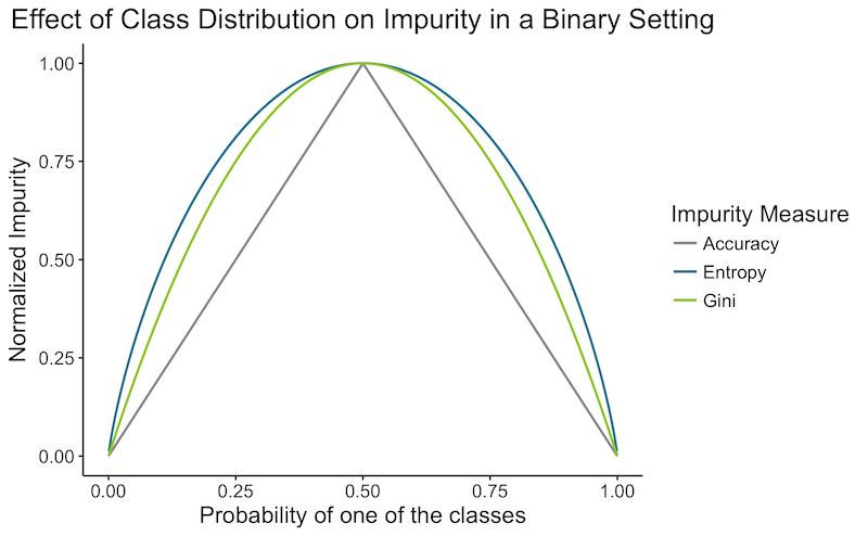
Here is a quick graph showing the impurity depending on a class distribution in a binary setting:

Side Notes :

• Classification error may seem like a natural choice, but don't get fooled by the appearances: it's generally worst than the 2 other methods:
  • It is "more" greedy than the others. Indeed, it only focuses on the current error, while Gini and Entropy try to make a purer split which will make subsequent steps easier. Suppose we have a binary classification with 100 observation in each class $(100,100)$. Let's compare a split which divides the data into $(20,80)$ and $(80,20)$, to an other split which would divide it into $(40,100)$ and $(60,0)$. In both case the accuracy error would be of $0.20\%$. But we would prefer the second case, which is pure and will not have to be split further. Gini impurity and the Entropy would correctly chose the latter.
  • Classification error takes only into account the most probable class. So having a split with 2 extremely probable classes will have a similar error to split with one extremely probable class and many improbable ones.
• Gini Impurity and Entropy differ less than 2% of the time as you can see in the plot above. Entropy is a little slower to compute due to the logarithmic operation.

When should we stop splitting? It is important not to split too many times to avoid over-fitting. Here are a few heuristics that can be used as a stopping criterion:

• When the number of training examples in a a leaf node is small.
• When the depth reaches a threshold.
• When the impurity is low.
• When the purity gain due to the split is small.

Such heuristics require problem-dependent thresholds (hyperparameters), and can yield relatively bad results. For example decision trees might have to split the data without any purity gain, to reach high purity gains at the following step. It is thus common to grow large trees using the number of training example in a leaf node as a stopping criterion. To avoid over-fitting, the algorithm would prune back the resulting tree. In CART, the pruning criterion $C_{pruning}(T)$ balances impurity and model complexity by regularization. The regularized variable is often the number of leaf nodes $\vert T \vert$, as below:

$\lambda$ is selected via cross validation and trades-off impurity and model complexity, for a given tree $T$, with leaf nodes $v=1…\vertT \vert$ using Impurity measure $I$.

Variants: there are various decision tree methods, that differ with regards to the following points:

• Splitting Criterion ? Gini / Entropy.
• Technique to reduce over-fitting ?
• How many variables can be used in a split ?
• Building binary trees ?
• Handling of missing values ?
• Do they handle regression?
• Robustness to outliers?

Famous variants:

• ID3: first decision tree implementation. Not used in practice.
• C4.5: Improvement over ID3 by the same developer. Error based pruning. Uses entropy. Handles missing values. Susceptible to outliers. Can create empty branches.
• CART: Uses Gini. Cost complexity pruning. Binary trees. Handles missing values. Handles regression. Not susceptible to outliers.
• CHAID: Finds a splitting variable using Chi-squared to test the dependency between a variable and a response. No pruning. Seems better for describing the data, but worst for predicting.

Other variants include : C5.0 (next version of C4.5, probably less used because it's patented), MARS.

Resources : A comparative study of different decision tree methods.

• Pseudocode The simple version of a decision tree can be written in a few lines of python pseudocode:

def buildTree(X,Y):
    if stop_criteria(X,Y) :
        # if stop then store the majority class
        tree.class = mode(X) 
        return Null

    minImpurity = infinity
    bestSplit = None
    for j in features:
        for T in thresholds:
            if impurity(X,Y,j,T) < minImpurity:
                bestSplit = (j,T)
                minImpurity = impurity(X,Y,j,T) 

    X_left,Y_Left,X_right,Y_right = split(X,Y,bestSplit)

    tree.split = bestSplit # adds current split
    tree.left = buildTree(X_left,Y_Left) # adds subsequent left splits
    tree.right buildTree(X_right,Y_right) # adds subsequent right splits

return tree

def singlePredictTree(tree,xi):
    if tree.class is not Null:
        return tree.class

    j,T = tree.split
    if xi[j] >= T:
        return singlePredictTree(tree.right,xi)
    else:
        return singlePredictTree(tree.left,xi)

def allPredictTree(tree,Xt):
    t,d = Xt.shape
    Yt = vector(d)
    for i in t:
        Yt[i] = singlePredictTree(tree,Xt[i,:])

    return Yt

• Complexity I will be using the following notation: \(M=depth\) ; \(K=\#_{thresholds}\) ; \(N = \#_{train}\) ; \(D = \#_{features}\) ; \(T = \#_{test}\) .

Let's first think about the complexity for building the first decision stump (first function call):

• In a decision stump, we loop over all features and thresholds $O(KD)$, then compute the impurity. The impurity depends solely on class probabilities. Computing probabilities means looping over all $X$ and count the $Y$ : $O(N)$. With this simple pseudocode, the time complexity for building a stump is thus $O(KDN)$.
• In reality, we don't have to look for arbitrary thresholds, only for the unique values taken by at least an example. E.g. no need of testing $feature_j>0.11$ and $feature_j>0.12$ when all $feature_j$ are either $0.10$ or $0.80$. Let's replace the number of possible thresholds $K$ by training set size $N$. $O(N^2D)$
• Currently we are looping twice over all $X$, once for the threshold and once to compute the impurity. If the data was sorted by the current feature, the impurity could simply be updated as we loop through the examples. E.g. when considering the rule $feature_j>0.8$ after having already considered $feature_j>0.7$, we do not have to recompute all the class probabilities: we can simply take the probabilities from $feature_j>0.7$ and make the adjustments knowing the number of example with $feature_j==0.7$. For each feature $j$ we should first sort all data $O(N\log(N))$ then loop once in $O(N)$, the final would be in $O(DN\log(N))$.

We now have the complexity of a decision stump. You could think that finding the complexity of building a tree would be multiplying it by the number of function calls: Right? Not really, that would be an over-estimate. Indeed, at each function call, the training data size $N$ would have decreased. The intuition for the result we are looking for, is that at each level $l=1…M$ the sum of the training data in each function is still $N$. Multiple function working in parallel with a subset of examples take the same time as a single function would, with the whole training set $N$. The complexity at each level is thus still $O(DN\log(N))$ so the complexity for building a tree of depth $M$ is $O(MDN\log(N))$. Proof that the work at each level stays constant:

At each iterations the dataset is split into $\nu$ subsets of $k_i$ element and a set of $n-\sum_{i=1}^{\nu} k_i$. At every level, the total cost would therefore be (using properties of logarithms and the fact that $k_i \le N$ ) :

The last possible adjustment I see, is to sort everything once, store it and simply use this precomputed data at each level. The final training complexity is therefore $O(MDN + ND\log(N))$ .

The time complexity of making predictions is straightforward: for each $t$ examples, go through a question at each $M$ levels. I.e. $O(MT)$ .