Dynamic programing

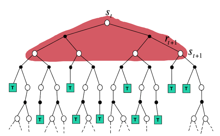
Side Notes: DP algorithms use the Bellman equations to update estimates based on other estimates (typically the value function at the next state). This general idea is called Bootstrapping.

Policy Iteration

The high-level idea is to iteratively: evaluate $v_\pi$ for the current policy $\pi$ (policy evaluation 1), use $v_\pi$ to improve $\pi'$ (policy improvement 1), evaluate $v_{\pi'}$ (policy evaluation 2)… Thus obtaining a sequence of strictly monotonically improving policies and value functions (except when converged to $\pi_{*}$). As a finite MDP has only a finite number of possible policies, this is guaranteed to converge in a finite number of steps. This idea is often visualized using a 1d example taken from Sutton and Barto):

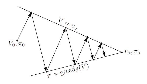
This simplified diagram shows that although the policy improvement and policy evaluation "pull in opposite directions", the 2 processes still converge to find a single joint solution. Almost all RL algorithms can be described using 2 interacting processes (the prediction task for approximating a value, and the control task for improving the policy), which are often called Generalized Policy Iteration (GPI).

In python pseudo-code:

def policy_iteration(environment):
    # v initialized arbitrarily for all states except V(terminal)=0
    v, pi = initialize()
    is_converged = False
    while not is_converged:
        v = policy_evaluation(pi, environment, v)
        pi, is_converged = policy_improvement(v, environment, pi)
    return pi

Policy Evaluation

The first step is to evaluate $v_\pi$ for a given $\pi$. This can be done by solving the Bellman equation :

Solving the equation can be done by either:

• Linear System: This is a set of linear equations ($\vert \mathcal{S} \vert$ equations and unknowns) with a unique solution (if $\gamma <1$ or if it is an episodic task). Note that we would have to solve for these equations at every step of the policy iteration and $\vert \mathcal{S} \vert$ is often very large. Assuming a deterministic policy and reward, this would take $O(\vert \mathcal{S} \vert^3)$ operations to solve.

• Iterative method: Modify the Bellman equation to become an iterative method that is guaranteed to converge when $k\to \infty$ if $v_\pi$ exists. This is done by realizing that $v_\pi$ is a fixed point of:

Side Notes : In the iterative method, we would have to keep to keep 2 arrays $v_k(s)$ and $v_{k+1}(s)$. At each iteration $k$ we would update $v_{k+1}(s)$ by looping through all states. Importantly, the algorithm also converges to $v_\pi(s)$ if we keep in memory a single array that would be updated "in-place" (often converges faster as it updates the value for some states using the latest available values). The order of state updates has a significant influence on the convergence in the "in-place" case .

We solve for an approximation $V \approx v_\pi$ by halting the algorithm when the change for every state is "small".

In python pseudo-code:

def q(s, a, v, environment, gamma):
    """Computes the action-value function `q` for a given state and action."""
    dynamics, states, actions, rewards = environment
    return sum(dynamics(s_p,r,s,a) * (r + gamma * v(s_p))
               for s_p in states
               for r in rewards)

def policy_evaluation(pi, environment, v_init, threshold=..., gamma=...):
    dynamics, states, actions, rewards = environment
    V = v_init # don't restart from scratch policy evaluation
    delta = 0
    while delta < threshold :
        delta = 0
        for s in states:
            v = V(s)
            # Bellman update
            V(s) = sum(pi(a, s) * q(a,s, V, environment, gamma) for s_p in states)
            # stop when change for any state is small
            delta = max(delta, abs(v-V(s)))
    return v

Policy Improvement

Now that we have an (estimate of) $v_\pi$ which says how good it is to be in $s$ when following $\pi$, we want to know how to change the policy to yield a higher return.

We have previously defined a policy $\pi'$ to be better than $\pi$ if $v_{\pi'}(s) > v_{\pi}(s), \forall s$. One simple way of improving the current policy $\pi$ would thus be to use a $\pi'$ which is identical to $\pi$ at each state besides one $s_{update}$ for which it will take a better action. Let's assume that we have a deterministic policy $\pi$ that we follow at every step besides one step when in $s_{update}$ at which we follow the new $\pi'$ (and continue with $\pi$). By construction :

Then it can be proved that (Policy Improvement Theorem) :

I.e. if such policy $\pi'$ can be constructed, then it is a better than $\pi$.

The same holds if we extend the update to all actions and all states and stochastic policies. The general policy improvement algorithm is thus :

$\pi'$ is always going to be better than $\pi$ except if $\pi=\pi_{*}$, in which case the update equations would turn into the Bellman optimality equation.

In python pseudo-code:

def policy_improvement(v, environment, pi):
    dynamics, states, actions, rewards = environment
    is_converged = True
    for s in states:
        old_action = pi(s)
        # q defined in `policy_evaluation` pseudo-code
        pi(s) = argmax(q(s,a, v, environment, gamma) for a in actions)
        if old_action != pi(s):
            is_converged = False
    return pi, is_converged

Practical : Assuming a deterministic reward, this would take $O(\vert \mathcal{S} \vert^2 \vert \mathcal{A} \vert)$ operations to solve. Each iteration of the policy iteration algorithm thus takes $O(\vert \mathcal{S} \vert^2 (\vert \mathcal{S} \vert + \vert \mathcal{A} \vert))$ for a deterministic policy and reward signal, if we solve the linear system of equations for the policy evaluation step.

Value Iteration

In policy iteration, the bottleneck is the policy evaluation which requires multiple loops over the state space (convergence only for an infinite number of loops). Importantly, the same convergence guarantees as with policy iteration hold when doing a single policy evaluation step. Policy iteration with a single evaluation step, is called value iteration and can be written as a simple update step that combines the truncated policy evaluation and the policy improvement steps:

This is guaranteed to converge for arbitrary $v_0$ if $v_*$ exists. Value iteration corresponds to the update rule derived from the Bellman optimality equation . The formula, is very similar to policy evaluation, but it maximizes instead of marginalizing over actions.

Like policy evaluation, value iteration needs an infinite number of steps to converge to $v_*$. In practice we stop whenever the change for all actions is small.

In python pseudo-code:

def value_to_policy(v, environment, gamma):
    """Makes a deterministic policy from a value function."""
    dynamics, states, actions, rewards = environment
    pi = dict()
    for s in states:
        # q defined in `policy_evaluation` pseudo-code
        pi(s) = argmax(q(s,a, v, environment, gamma) for a in actions)
    return pi

def value_iteration(environment, threshold=..., gamma=...):
    dynamics, states, actions, rewards = environment
    # v initialized arbitrarily for all states except V(terminal)=0
    V = initialize()
    delta = threshold + 1 # force at least 1 pass 
    while delta < threshold :
        delta = 0
        for s in states:
            v = V(s)
            # Bellman optimal update
            # q defined in `policy_evaluation` pseudo-code
            V(s) = max(q(s, a, v, environment, gamma) for a in actions)
            # stop when change for any state is small
            delta = max(delta, abs(v-V(s)))
    pi = value_to_policy(v, environment, gamma)
    return pi

Practical : Faster convergence is often achieved by doing a couple of policy evaluation sweeps (instead of a single one in the value iteration case) between each policy improvement. The entire class of truncated policy iteration converges. Truncated policy iteration can be schematically seen as using the modified generalized policy iteration diagram:

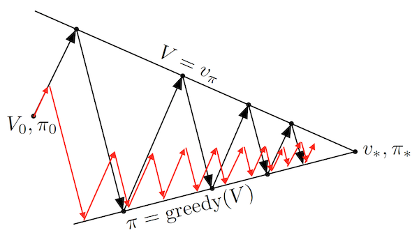
As seen above, truncated policy iteration uses only approximate value functions. This usually increases the number of required policy evaluation and iteration steps, but greatly decreases the number of steps per policy iteration making the overall algorithm usually quicker. Assuming a deterministic policy and reward signal, each iteration for the value iteration takes $O(\vert \mathcal{S} \vert^2 \vert \mathcal{A} \vert)$ which is less than exact (solving the linear system) policy iteration $O(\vert \mathcal{S} \vert^2 (\vert \mathcal{S} \vert + \vert \mathcal{A} \vert))$.

Asynchronous Dynamic Programming

A drawback of DP algorithms, is that they require to loop over all states for a single sweep. Asynchronous DP algorithms are in-place iterative methods that update the value of each state in any order. Such algorithms are still guaranteed to converge as long as it can't ignore any state after some points (for the episodic case it is also easy to avoid the few orderings that do not converge).

By carefully selecting the states to update, we can often improve the convergence rate. Furthermore, asynchronous DP enables to update the value of the states as the agent visits them. This is very useful in practice, and focuses the computations on the most relevant states.

Practical : Asynchronous DP are usually preferred for problems with large state-spaces

Non DP Exact Methods

Although DP algorithms are the most used for finding exact solution of the Bellman optimality equations, other methods can have better worst-case convergence guarantees. Linear Programming (LP) is one of those methods. Indeed, the Bellman optimality equations can be written as a linear program. Let $B$ be the Bellman operator (i.e. $v_{k+1} = B(v_k)$), and $\pmb{\mu_0}$ is a probability distribution over states, then:

Indeed, if $v \geq B(v)$ then $B(v) \geq B(B(v))$ due to the monotonicity of the Bellman operator. By repeated applications we must have that $v \geq B(v) \geq B(B(v)) \geq B^3(v) \geq \ldots \geq B^{\infty}(v) = v_{*}$. Any solution of the LP must satisfy $v \geq B(v)$ and must thus be $v_{*}$. Then the objective function $\pmb{\mu}_0^T \mathbf{v}$ is the expected cumulative reward when beginning at a state drawn from $\pmb{\mu}_0$. By substituting for the Bellman operator $B$:

Using the dual form of the LP program, the equation above can be rewritten as :

The constraints in the dual LP ensure that :

I.e. they are the discounted state-action counts. While the dual objective maximizes the expected discounted return. The optimal policy can is :

$\pi_*(s)=max_a \mu(s,a)$

Practical: Linear programming is sometimes better than DP for small number of states, but it does not scale well.

Although LP are rarely useful, they provide connections to a number of other methods that have been used to find approximate large-scale MDP solutions.