Monte Carlo GPI

As mentioned previously, the dynamics of the environment are rarely known. In such cases we cannot use DP. Monte Carlo (MC) methods bypass this lack of knowledge by estimating the expected return from experience (i.e. sampling of the unknown dynamics).

MC methods are very similar to the previously discussed Generalized Policy Iteration(GPI). The main differences being:

• They learn the value-function by sampling from the MDP (experience) rather than computing these values using the dynamics of the MDP.

• MC methods do not bootstrap: each value function for each state/action is estimated independently. I.e. they do not update value estimates based on other value estimates.

• In DP, given a state-value function, we could look ahead one step to determine a policy. This is not possible anymore due to the lack of knowledge of the dynamics. It is thus crucial to estimate the action value function $q_{*}$ instead of $v_{*}$ in policy evaluation.

Recall that $q_\pi(s) = \mathbb{E}[R_{t+1} + \gamma G_{t+1} \vert S_{t}=s, A_t=a]$. Monte Carlo Estimation approximates this expectations through sampling. I.e. by averaging the returns after every visits of state action pairs $(s,a)$.

Note that pairs $(s,a)$ could be visited multiple times in the same episode. How we treat these visits gives rise to 2 slightly different methods:

• First-visit MC Method: estimate $q_\pi(s,a)$ as the average of the returns following the first visit to $(s,a)$. This has been more studied and is the one I will be using.
• Every-visit MC Method: estimate $q_\pi(s,a)$ as the average of the returns following all visit to $(s,a)$. These are often preferred as they don't require to keep track of which states have been visited.

Both methods converge to $q_\pi(s,a)$ as the number of visits $n \to \infty$. The convergence of the first-visit MC is easier to prove as each return is an i.i.d estimate of $q_\pi(s,a)$. The standard deviation of the estimate drops with $\frac{1}{\sqrt{n}}$.

Side Notes:

• MC methods can learn from actual experience or simulated one. The former is used when there's no knowledge about the dynamics. The latter is useful when it is possible to generate samples of the environment but infeasible to write it explicitly. For example, it is very easy to simulate a game of blackjack, but computing $p(s',r' \vert s,a)$ as a function of the dealer cards is complicated.
• The return at each state depends on the future action. Due to the training of the policy, the problem becomes non-stationary from the point of view of the earlier states.
• In order to have well defined returns, we will only be considering episodic tasks (i.e. finite $T$)
• The idea is the same as in Bayesian modeling, where we approximated expectations by sampling.
• MC methods do not bootstrap and are thus very useful to compute the value of only a subset of states, by starting many episodes at the state of interests.

On-Policy Monte Carlo GPI

Let's make a simple generalized policy iteration (GPI) algorithm using MC methods. As a reminder, GPI consists in iteratively alternating between evaluation (E) and improvement (I) of the policy, until we reach the optimal policy:

• Generalized Policy Evaluation (prediction). Evaluates the value function $Q \approx q_\pi$ (not $V$ as we do not have the dynamics). Let $F_i(s,a)$ return the time step $t$ at which state-action pair $(s,a)$ is first seen (first-visit MC) in episode $i$ (return $-1$ if never seen), and $G_{t}^{(i)}(\pi)$ be the discounted return from time $t$ of the $i^{th}$ episode when following $\pi$:

• Policy Improvement, make a GLIE (defined below) policy $\pi$ from $Q$. Note that the policy improvement theorem still holds.

Unsurprisingly, MC methods can be shown to converge if they maintain exploration and when the policy evaluation step uses an $\infty$ number of samples. Indeed, these 2 conditions ensure that all expectations are correct as MC sampling methods are unbiased.

Of course using an $\infty$ number of samples is not possible, and we would like to alternate (after every episode) between evaluation and improvement even when evaluation did not converge (similarly value iteration). Although MC methods cannot converge to a suboptimal policy in this case, the fact that it converges to the optimal fixed point has yet to be formally proved.

Maintaining exploration is a major issue. Indeed, if $\pi$ is deterministic then the samples will only improve estimates for one action per state. To ensure convergence we thus need a policy which is Greedy in the Limit with Infinite Exploration (GLIE). I.e. : 1/ All state-action pairs have to be explored infinitely many times; 2/ The policy has to converge to a greedy one. Possible solutions include:

• Exploring Starts: start every episode with a sampled state-action pair from a distribution that is non-zero for all pairs. This ensures that all pairs $(s,a)$ will be visited an infinite number of times as $n \to \infty$. Choosing starting conditions is often not applicable (e.g. most games always start from the same position).
• Non-Zero Stochastic Policy: to ensure that all pairs $(s,a)$ are encountered, use a stochastic policy with a non-zero probability for all actions in each state. $\epsilon\textbf{-greedy}$ is a well known policy, which takes the greedy action with probability $1-(\epsilon+\frac{\epsilon}{\vert \mathcal{A} \vert})$ and assigns a uniform probability of $\frac{\epsilon}{\vert \mathcal{A} \vert}$ to all other actions. To be a GLIE policy, $\epsilon$ has to converge to 0 in the limit (e.g. $\frac{1}{t}$).

In python pseudo-code:

def update_eps_policy(Q, pi, s, actions, eps):
    """Update an epsilon policy for a given state."""
    q_best = -float("inf")
    for a in actions:
        pi[(a, s)] = eps/len(actions)
        q_a = Q[(s, a)]
        if q_a  > q_best:
            q_best = q_a 
            a_best = a
    pi[(a_best, s)] = 1 - (eps - (eps/len(actions)))
    return pi

def q_to_eps_pi(Q, eps, actions, states):
    """Creates an epsilon policy from a action value function."""
    pi = defaultdict(lambda x: 0)
    for s in states:
        pi = update_eps_policy(Q, pi, s, actions, eps)
    return pi

def on_policy_mc(game, actions, states, n=..., eps=..., gamma=...):
    """On policy Monte Carlo GPI using first-visit update and epsilon greedy policy."""
    returns = defaultdict(list)
    Q = defaultdict(lambda x: 0)
    for _ in range(n):
        pi = q_to_eps_pi(Q, eps, actions, states)
        T, list_states, list_actions, list_rewards = game(pi)
        G = 0
        for t in range(T-1,-1,-1): # T-1, T-2, ... 0
            r_t, s_t, a_t = list_rewards[t], list_states[t], list_actions[t]
            G = gamma * G + r_t # current return
            if s_t not in list_states[:t]: # if first
                returns[(s_t, a_t)].append(G)
                Q[(s_t, a_t)] = mean(returns[(s_t, a_t)]) # mean over all episodes
    return V

Incremental Implementation

The MC methods can be implemented incrementally. Instead of getting estimates of $q_\pi$ by keeping in memory all $G_t^{(i)}$ to average over those, the average can be computed exactly at each step $n$. Let $m := \sum_i \mathcal{I}[F_i(s,a) \neq -1]$, then:

This is of the general form :

Where the step-size $\alpha_n$ varies as it is $\frac{1}{n}$. In RL, problems are often non-stationary, in which case we would like to give more importance to recent samples. A popular way of achieving this, is by using a constant step-size $\alpha \in ]0,1]$. This gives rise to an exponentially decaying weighted average (also called exponential recency-weighted average in RL). Indeed:

Intuition: At every step we update our estimates by taking a small step towards the goal, the direction (sign in 1D) is given by the error $\epsilon = \left(G_{F_m(s,a)}^{(m)}(\pi) - Q_{n}(s,a) \right)$ and the steps size by $\alpha * \vert \epsilon \vert$.

Side Notes:

• The weight given the $i^{th}$ return $G_{F_i(s,a)}^{(i)}(\pi)$ is $\alpha(1-\alpha)^{n-i}$, which decreases exponentially as i decreases ($(1-\alpha) \in [0,1[$).
• It is a well weighted average because the sum of the weights can be shown to be 1.
• From stochastic approximation theory we know that we need a Robbins-Monro sequence of $\alpha_n$ for convergence: $\sum_{m=1}^{\infty} \alpha_m = \infty$ (steps large enough to overcome initial conditions / noise) and $\sum_{m=1}^{\infty} \alpha_m^2 < \infty$ (steps small enough to converge). This is the case for $\alpha_m = \frac{1}{m}$ but not for a constant $\alpha$. But in non-stationary environment we actually don't want the algorithm to converge, in order to continue learning.
• For every-visit MC, this can simply be rewritten as the following update step at the end of each episode:

Off-Policy Monte Carlo GPI

In the on-policy case we had to use a hack ($\epsilon \text{-greedy}$ policy) in order to ensure convergence. The previous method thus compromises between ensuring exploration and learning the (nearly) optimal policy. Off-policy methods remove the need of compromise by having 2 different policy.

The behavior policy $b$ is used to collect samples and is a non-zero stochastic policy which ensures convergence by ensuring exploration. The target policy $\pi$ is the policy we are estimating and will be using at test time, it focuses on exploitation. The latter is often a deterministic policy. These methods contrast with on-policy ones, that uses a single policy.

Intuition: The intuition behind off-policy methods is to follow an other policy but to weight the final return in such a way that compensates for the actions taken by $b$. This can be done via Importance Sampling without biasing the final estimate.

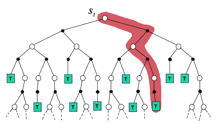
Given a starting state $S_t$ the probability of all subsequent state-action trajectory $A_t, S_{t+1}, A_{t+1}, \ldots, S_T$ when following $\pi$ is:

Note that the dynamics $p(s' \vert s, a)$ are unknown but we only care about the ratio of the state-action trajectory when following $\pi$ and $b$. The importance sampling ratio is:

Note that if we simply average over all returns we would get $\mathbb{E}[G_t \vert S_t=s] = v_b(s)$, to get $v_\pi(s)$ we can use the previously computed importance sampling ratio:

Side Notes:

• Off policy methods are more general as on policy methods can be written as off-policy methods with the same behavior and target policy.
• In order to estimate values of $\pi$ using $b$ we require $\pi(a \vert s) \ge 0 \implies b(a\vert s) \ge$ (coverage assumption). I.e. all actions of $\pi$ can be taken by $b$.
• The formula shown above is the ordinary importance sampling, although it is unbiased it can have large variance. Weighted importance sampling is biased (although it is a consistent estimate as the bias decreases with $O(1/n)$) but is usually preferred as the variance is usually dramatically smaller:

• The importance method above treats the returns $G_0$ as a whole, without taking into account the discount factors. For example if $\gamma=1$, then $G_0 = R_1$, we would thus only need the importance sampling ratio $\frac{pi(A_0 \vert S_0)}{b(A_0 \vert S_0)}$, yet we currently use also the 99 other factors $\frac{pi(A_1 \vert S_1)}{b(A_1 \vert S_1)} \ldots \frac{pi(A_{99} \vert S_{99})}{b(A_{99} \vert S_{99})}$ which greatly increases the variance. Discounting-aware importance sampling greatly decreases the variance by taking the discounts into account.

Practical: Off-policy methods are very useful to learn by seeing a human expert or non-learning controller.

In python pseudo-code:

def off_policy_mc(Q, game, b, actions, n=..., gamma=...):
    """Off policy Monte Carlo GPI using incremental update and weighted importance sampling."""
    pi = dict()
    returns = defaultdict(list)
    Q = defaultdict(lambda x: random.rand)
    C = defaultdict(lambda x: 0)
    for _ in range(n):
        T, list_states, list_actions, list_rewards = game(b)
        G = 0
        W = 1
        for t in range(T-1,-1,-1): # T-1, T-2, ... 0
            r_t, s_t, a_t = list_rewards[t], list_states[t], list_actions[t]
            G = gamma * G + r_t # current return
            C[(s_t, a_t)] += W
            Q[(s_t, a_t)] += (W/C[(s_t, a_t)])(G-Q[(s_t, a_t)])
            pi[s_t] = argmax(Q[(s_t, a)] for a in actions)
            if a_t != pi(s):
                break
            W /= b[(s_t, a_t)]
    return V

Side Notes: As for on policy, Off policy MC control can also be written in an Incremental manner. The details can be found in chapter 5.6 of Sutton and Barto.