Variational autoencoder

Deep Learning Perspective

A VAE can be thought of an auto-encoder that maps and reconstructs inputs to and from latent distributions rather than point-wise latent codes. This enables sampling to generate new examples and forces similar examples to be encoded by similar latent distributions. Indeed, latent distributions with more overlap or forced to generate similar samples. Importantly, making the network generate noise around the latent point-wise estimates is not satisfactory as the encoder would learn to generate very large means or very small variance, thus making the noise neglectable. To avoid this issue we force the latent distributions to be close to a given distribution $p(\mathbf{z})$ (typically a unit Gaussian).

The encoder is a neural network parametrized by $\mathbf{\phi}$ that maps the input $\mathbf{x}$ to a latent distribution $q_\phi(\mathbf{z}\vert\mathbf{x})$ from which to sample a noisy representations of the low dimension latent code $\mathbf{z}$. The decoder is parametrized by $\mathbf{\theta}$ and deterministically maps the sampled latent code $\mathbf{z}$ to the corresponding reconstructed $\mathbf{\hat{x}}=f_\theta(\mathbf{z})$. The training procedure requires to minimize the expected reconstruction loss $L(\mathbf{x},\mathbf{\hat{x}})$ under the constraint of having $q_\phi(\mathbf{z}\vert \mathbf{x}) \approx p(\mathbf{z})$. The latter constraint can be written as $D_\text{KL}(q_\phi(\mathbf{z}\vert\mathbf{x})\parallel p(\mathbf{z}) ) < \delta$

This constrained optimization problem can be rewritten as an unconstrained one using the KKT conditions (generalization of Lagrange multipliers allowing inequality constraints):

Where the last line replaced the reconstruction loss $L$ with the negative log likelihood of the data as predicted by a hypothetical probabilistic discriminator. The output of the deterministic discriminator can be interpreted as the expected value of the hypothetical probabilistic discriminator. Many of the usual losses $L$ for deterministic outputs correspond to negative log likelihoods: mean squared error <-> Gaussian likelihood, log loss <-> logistic likelihood,…

The global loss consists of the expected reconstruction loss (first term) and a regularisation term (KL divergence).

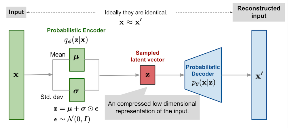
We now have a loss and a model: it should be straight-forward to train such a network in your favorite deep learning library, right ? Not really… The problem arises from the stochasticity of the latent representation $\mathbf{z}\sim q_\phi(\mathbf{z}\vert\mathbf{x})$. Indeed, during the backward pass, gradients cannot flow through stochastic nodes. Fortunately, there's a simple way of making it work by using the reparametrisation trick, which consists in expressing $\mathbf{z}$ as a deterministic function of the inputs and of an independent random variable $\mathbf{z}=g_\phi(\mathbf{x}, \pmb{\epsilon})$. In the case of a multivariate Gaussian with a diagonal covariance, the following equations are equivalent:

The figure from Lil'Log summarizes very well the deep learning point of view, with the small caveat that in practice we use a deterministic decoder and a loss function rather than the probabilistic one:

Side Notes :

• The loss corresponds to $\beta$-VAE. You recover the original VAE loss by setting $\beta=1$.

• Usually $p(\mathbf{z})=\mathcal{N}(\mathbf{z};\mathbf{0},I)$ and $q_\phi(\mathbf{z}\vert\mathbf{x})=\mathcal{N}(\mathbf{z};\pmb{\mu}(\mathbf{x}),\text{diag}(\pmb{\sigma}(\mathbf{x})))$. In which case the KL divergence can be computed in closed form :

• In practice, it is better to make the network output $\log \, \pmb{\sigma^2}$ (the log variance) as this constrains sigma to be positive even with the network outputting a real value. We output the variance instead of $\pmb{\sigma}$ as it shows up twice in the KL divergence.

• For black and white image generation (e.g. MNIST), cross-entropy loss (corresponding to fitting a Bernouilli for each pixel) gives better results than mean squared error. It is often also used for colored images by rescaling each pixel from $[0,255]$ to $[0,1]$. Note that using a Gaussian distribution would make sense as there's no reason to penalize differently $(0.1, 0.2)$ and $(0.5, 0.6)$, but MSE loss ends up focusing only a few pixels that are very wrong.

Graphical Model Perspective

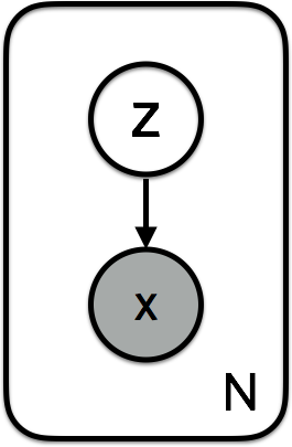
When defining a generative probabilistic model, it is important to define a step by step generation procedure. For each datapoint $i$:

1. Sample the latent variable (i.e. the semantics of what you want to generate): $\mathbf{z}^{(n)} \sim p(\mathbf{z})$.
2. Sample the generated datapoint conditioned on the latent variable: $\mathbf{x}^{(n)} \sim p(\mathbf{x} \vert \mathbf{z})$.

The graphical model is simply :

The objective is to have a graphical model that maximizes the probability of generating real data :

Unfortunately the integral above is not tractable, as it would require integrating over all possible $\mathbf{z}$ sampled from a prior. It could be approximated by Markov Chain Monte Carlo (MCMC), i.e. by sampling $N$ different $\mathbf{z}^{(n)}$ and then compute $p(\mathbf{x}) \approx \frac{1}{N}\sum_{n=1}^{N}p(\mathbf{x}\vert\mathbf{z}^{(n)})$. But as the volume spanned by $\mathbf{z}$ is potentially large, $N$ may need to be very large to obtain an accurate estimate of $p(\mathbf{x})$ (as we will sample many times from uninformative regions of the prior). To improve the sample efficiency (decrease variance) of the estimate we would like to sample "important" $\mathbf{z}$ rather than blindly sampling from the prior. Let's call $q$ a probability distribution that assigns high probability to "important" $\mathbf{z}$. As the notion of "importance" might depend on the $\mathbf{x}$ we want to predict, let's condition $q$ on those : $q(\mathbf{z} \vert \mathbf{x})$. We can use Importance Sampling to use samples from $q(\mathbf{z} \vert \mathbf{x})$ without biasing our estimate:

Noting that $-\log$ is a convex function, we can use Jensen Inequality, which states that $g(\mathbb{E}[X]) \leq \mathbb{E}[g(X)] \text{, where } g \text{ is convex}$:

The right hand side of the equation is called the Evidence Lower Bound (ELBO) as it lower bounds the (log) evidence $p(\mathbf{x})$. The last missing component is to chose appropriate probability functions :

• $p(\mathbf{x} \vert \mathbf{z})$ might be a very complicated distribution. We use a neural network parametrized by $\pmb{\theta}$ to approximate it: $p_\theta(\mathbf{x} \vert \mathbf{z})$.
• $p(\mathbf{z})$ can be any prior. It is often set as $\mathcal{N}(\mathbf{0}, I)$ which makes the KL divergence term simple and states that we prefer having latent codes with uncorrelated dimensions (disentangled).
• $q(\mathbf{z}\vert \mathbf{x})$ should give more mass to "important" $\mathbf{z}$. We let a neural network parametrized by $\pmb{\phi}$ deciding how to set it : $q_\phi(\mathbf{z} \vert \mathbf{x})$. In order to have a closed form KL divergence, we usually use a Gaussian distribution with diagonal covariance whose parameters $\pmb{\mu}, \pmb{\sigma}$ are the output of the neural network : $q_\phi(\mathbf{z} \vert \mathbf{x}) = \mathcal{N}(\mathbf{z};\pmb{\mu}(\mathbf{x}),\text{diag}(\pmb{\sigma}(\mathbf{x})))$.

Finally, let's train $\pmb{\theta}$ and $\pmb{\phi}$ by maximizing the probability of generating the training (i.e. real) data $p_{\theta,\phi}(\mathbf{x})$. Assuming that all data points are i.i.d then:

This corresponds to the loss we derived with the deep learning perspective for $\beta=1$ (the signs are versed because we are maximizing instead of minimizing). Please refer to the previous subsection for the reparamatrization trick and closed form solution of the KL divergence.

Side Notes :

• The ELBO can also be derived by directly minimizing $D_\text{KL}(q(\mathbf{z} \vert \mathbf{x}) \parallel p(\mathbf{z} \vert \mathbf{x}) )$, which intuitively "turns the problem around" and tries to find a good mapping from $\mathbf{x}$ to $\mathbf{z}$. The idea of doing approximate tractable inference with a simple distribution $q(\mathbf{z} \vert \mathbf{x})$ instead of the real posterior $p(\mathbf{z} \vert \mathbf{x})$ is called variational inference. This is where the name of variational auto-encoder comes from.

• The choice of direction of the KL divergence is natural with the importance sampling derivation.

• You can get a tighter lower bound by getting a less biased estimate of the expectation you want, by using sampling methods: $\mathbb{E}_{q(\mathbf{z}\vert \mathbf{x})} \left[ \log \left( p(\mathbf{x} \vert \mathbf{z}) \frac{p(\mathbf{z})}{q(\mathbf{z}\vert \mathbf{x})} \right) \right]$. In expectation this is a tighter lower bound is called Importance Weighted Autoencoders.

Resources : D. Kingma and M. Welling first paper on VAEs

Intuition: Disentangled Representations

Disentangled representations most often refers to having a latent space where with each dimension is not very correlated (factorizable latent space). Such representations have been shown to be more general and robust. They enable compositionality, which is key for human thoughts and language. For example, if I ask you to draw a blue apple, you would not have any issues doing it (assuming your drawing skills are better than mine ) because you understand the concept of an apple and the concept of being blue. Being able to model such representation is what we are aiming for in VAE, as illustrated in Jeremy Jordan's blog :

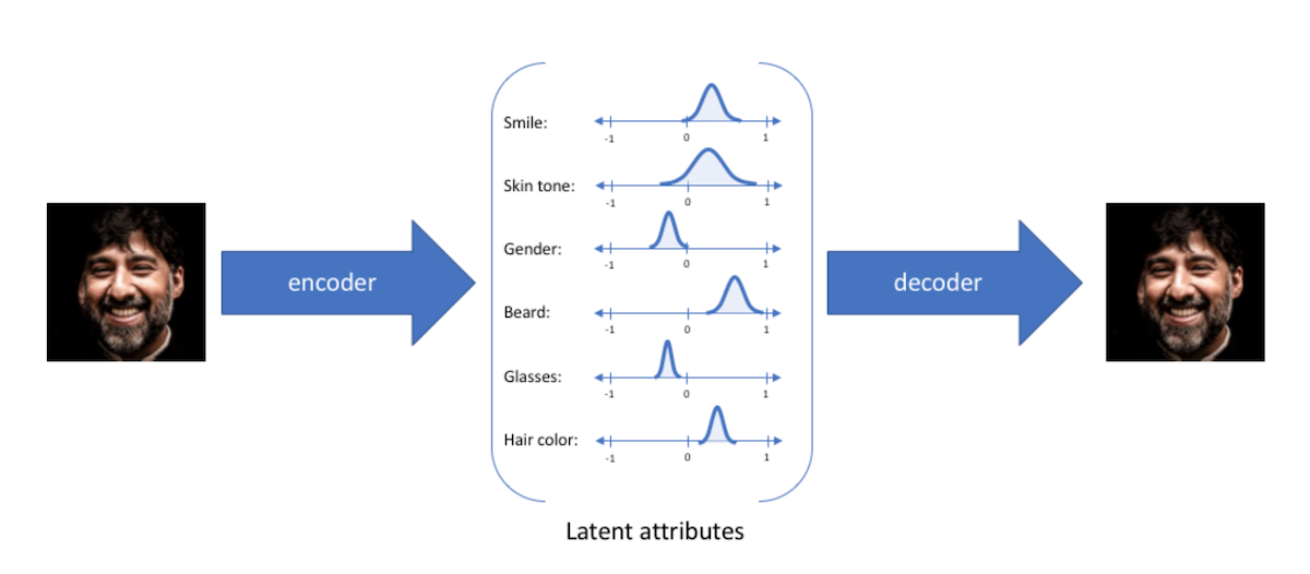
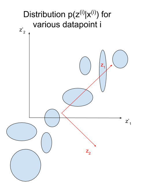
Having Gaussian distribution with diagonal covariance for the latent variable, means that each latent dimension can be modeled by a single Gaussian. Intuitively, we can thus think of latent dimensions as knobs used to add or remove something. Using a prior, forces the model to encode the confidence of how much of the knob to turn.

Although the variance of each knob is independent (diagonal covariance), the means can still be highly dependent. The unit Gaussian prior forces each dimension to correspond to the principle components of the distribution of means (i.e. the axes are parallel to the directions with the most variance like in PCA), thus forcing the knobs to encode disentangled factors of variations (small correlation) which are often more interpretable. This is because dimensions aligned with the principle components will decrease the KL divergence due to Pythagoras theorem. Graphically :