Naive Bayes
Overview
-
 Intuition :
- In the discrete case: "advance counting". E.g. Given a sentence $x_i$ to classify as spam or not, count all the times each word $w^i_j$ was in previously seen spam sentence and predict as spam if the total (weighted) "spam counts" is larger than the number of "non spam counts".
- Use a conditional independence assumption ("naive") to have better estimates of the parameters even with little data.
-
 Practical :
- Good and simple baseline.
- Thrive when the number of features is large but the dataset size is not.
- Training Complexity : $O(ND)$ .
- Testing Complexity : $O(TDK)$ .
- Notation Used : \(N= \#_{train}\) ; \(K= \#_{classes}\) ; \(D= \#_{features}\) ; \(T= \#_{test}\).
-
 Advantage :
- Simple to understand and implement.
- Fast and scalable (train and test).
- Handles online learning.
- Works well with little data.
- Not sensitive to irrelevant features.
- Handles real and discrete data.
- Probabilistic.
- Handles missing value.
-
 Disadvantage :
- Strong conditional independence assumption of features given labels.
- Sensitive to features that have not often been seen (mitigated by smoothing).
Naive Bayes is a family of generative models that predicts $p(y=c \vert\mathbf{x})$ by assuming that all features are conditionally independent given the label: $x_i \perp x_j \vert y , \forall i,j$. This is a simplifying assumption that very rarely holds in practice, which makes the algorithm "naive". Classifying with such an assumption is very easy:
\[\begin{aligned} \hat{y} &= arg\max_c p(y=c\vert\mathbf{x}, \pmb\theta) \\ &= arg\max_c \frac{p(y=c, \pmb\theta)p(\mathbf{x}\vert y=c, \pmb\theta) }{p(x, \pmb\theta)} & & \text{Bayes Rule} \\ &= arg\max_c \frac{p(y=c, \pmb\theta)\prod_{j=1}^D p(x_\vert y=c, \pmb\theta) }{p(x, \pmb\theta)} & & \text{Conditional Independence Assumption} \\ &= arg\max_c p(y=c, \pmb\theta)\prod_{j=1}^D p(x_j\vert y=c, \pmb\theta) & & \text{Constant denominator} \end{aligned}\]Note that because we are in a classification setting $y$ takes discrete values, so $p(y=c, \pmb\theta)=\pi_c$ is a categorical distribution.
You might wonder why we use the simplifying conditional independence assumption. We could directly predict using $\hat{y} = arg\max_c p(y=c, \pmb\theta)p(\mathbf{x} \vert y=c, \pmb\theta)$. The conditional assumption enables us to have better estimates of the parameters $\theta$ using less data . Indeed, $p(\mathbf{x} \vert y=c, \pmb\theta)$ requires to have much more data as it is a $D$ dimensional distribution (for each possible label $c$), while $\prod_{j=1}^D p(x_j \vert y=c, \pmb\theta)$ factorizes it into $D$ 1-dimensional distributions which requires a lot less data to fit due to curse of dimensionality. In addition to requiring less data, it also enables to easily mix different family of distributions for each features.
We still have to address 2 important questions:
- What family of distribution to use for $p(x_j \vert y=c, \pmb\theta)$ (often called the event model of the Naive Bayes classifier)?
- How to estimate the parameters $\theta$?
Event models of Naive Bayes
The family of distributions to use is an important design choice that will give rise to specific types of Naive Bayes classifiers. Importantly the family of distribution $p(x_j \vert y=c, \pmb\theta)$ does not need to be the same $\forall j$, which enables the use of very different features (e.g. continuous and discrete). In practice, people often use Gaussian distribution for continuous features, and Multinomial or Bernoulli distributions for discrete features :
Gaussian Naive Bayes :
Using a Gaussian distribution is a typical assumption when dealing with continuous data $x_j \in \mathbb{R}$. This corresponds to assuming that each feature conditioned over the label is a univariate Gaussian:
\[p(x_j \vert y=c, \pmb\theta) = \mathcal{N}(x_j;\mu_{jc},\sigma_{jc}^2)\]Note that if all the features are assumed to be Gaussian, this corresponds to fitting a multivariate Gaussian with a diagonal covariance : $p(\mathbf{x} \vert y=c, \pmb\theta)= \mathcal{N}(\mathbf{x};\pmb\mu_{c},\text{diag}(\pmb\sigma_{c}^2))$.
The decision boundary is quadratic as it corresponds to ellipses (Gaussians) that intercept .
Multinomial Naive Bayes :
In the case of categorical features $x_j \in \{1,…, K\}$ we can use a Multinomial distribution, where $\theta_{jc}$ denotes the probability of having feature $j$ at any step of an example of class $c$ :
\[p(\pmb{x} \vert y=c, \pmb\theta) = \operatorname{Mu}(\pmb{x}; \theta_{jc}) = \frac{(\sum_j x_j)!}{\prod_j x_j !} \prod_{j=1}^D \theta_{jc}^{x_j}\]Multinomial Naive Bayes is typically used for document classification , and corresponds to representing all documents as a bag of word (no order). We then estimate (see below)$\theta_{jc}$ by counting word occurrences to find the proportions of times word $j$ is found in a document classified as $c$.
The equation above is called Naive Bayes although the features $x_j$ are not technically independent because of the constraint $\sum_j x_j = const$. The training procedure is still the same because for classification we only care about comparing probabilities rather than their absolute values, in which case Multinomial Naive Bayes actually gives the same results as a product of Categorical Naive Bayes whose features satisfy the conditional independence property.
Multinomial Naive Bayes is a linear classifier when expressed in log-space :
\[\begin{aligned} \log p(y=c \vert \mathbf{x}, \pmb\theta) &\propto \log \left( p(y=c, \pmb\theta)\prod_{j=1}^D p(x_j \vert y=c, \pmb\theta) \right)\\ &= \log p(y=c, \pmb\theta) + \sum_{j=1}^D x_j \log \theta_{jc} \\ &= b + \mathbf{w}^T_c \mathbf{x} \\ \end{aligned}\]Multivariate Bernoulli Naive Bayes:
In the case of binary features $x_j \in \{0,1\}$ we can use a Bernoulli distribution, where $\theta_{jc}$ denotes the probability that feature $j$ occurs in class $c$:
\[p(x_j \vert y=c, \pmb\theta) = \operatorname{Ber}(x_j; \theta_{jc}) = \theta_{jc}^{x_j} \cdot (1-\theta_{jc})^{1-x_j}\]Bernoulli Naive Bayes is typically used for classifying short text , and corresponds to looking at the presence and absence of words in a phrase (no counts).
Multivariate Bernoulli Naive Bayes is not the same as using Multinomial Naive Bayes with frequency counts truncated to 1. Indeed, it models the absence of words in addition to their presence.
Training
Finally we have to train the model by finding the best estimated parameters $\hat\theta$. This can either be done using pointwise estimates (e.g. MLE) or a Bayesian perspective.
Maximum Likelihood Estimate (MLE):
The negative log-likelihood of the dataset $\mathcal{D}=\{\mathbf{x}^{(n)},y^{(n)}\}_{n=1}^N$ is :
\[\begin{aligned} NL\mathcal{L}(\pmb{\theta} \vert \mathcal{D}) &= - \log \mathcal{L}(\pmb{\theta} \vert \mathcal{D}) \\ &= - \log \prod_{n=1}^N \mathcal{L}(\pmb{\theta} \vert \mathbf{x}^{(n)},y^{(n)}) & & \textit{i.i.d} \text{ dataset} \\ &= - \log \prod_{n=1}^N p(\mathbf{x}^{(n)},y^{(n)} \vert \pmb{\theta}) \\ &= - \log \prod_{n=1}^N \left( p(y^{(n)} \vert \pmb{\pi}) \prod_{j=1}^D p(x_{j}^{(n)} \vert\pmb{\theta}_j) \right) \\ &= - \log \prod_{n=1}^N \left( \prod_{c=1}^C \pi_c^{\mathcal{I}[y^{(n)}=c]} \prod_{j=1}^D \prod_{c=1}^C p(x_{j}^{(n)} \vert \theta_{jc})^{\mathcal{I}[y^{(n)}=c]} \right) \\ &= - \log \left( \prod_{c=1}^C \pi_c^{N_c} \prod_{j=1}^D \prod_{c=1}^C \prod_{n : y^{(n)}=c} p(x_{j}^{(n)} \vert \theta_{jc}) \right) \\ &= - \sum_{c=1}^C N_c \log \pi_c + \sum_{j=1}^D \sum_{c=1}^C \sum_{n : y^{(n)}=c} \log p(x_{j}^{(n)} \vert \theta_{jc}) \\ \end{aligned}\]As the negative log likelihood decomposes in terms that only depend on $\pi$ and each $\theta_{jc}$ we can optimize all parameters separately.
Minimizing the first term by using Lagrange multipliers to enforce $\sum_c \pi_c$, we get that $\hat\pi_c = \frac{N_c}{N}$. Which is naturally the proportion of examples labeled with $y=c$.
The $\theta_{jc}$ depends on the family of distribution we are using. In the Multinomial case it can be shown to be $\hat\theta_{jc}=\frac{N_{jc}}{N_c}$. Which is very easy to compute, as it only requires to count the number of times a certain feature $x_j$ is seen in an example with label $y=c$.
Bayesian Estimate:
The problem with MLE is that it over-fits. For example, if a feature is always present in all training samples (e.g. the word "the" in document classification) then the model will break if it sees a test sample without that features as it would give a probability of 0 to all labels.
By taking a Bayesian approach, over-fitting is mitigated thanks to priors. In order to do so we have to compute the posterior :
\[\begin{aligned} p(\pmb\theta \vert \mathcal{D}) &= \prod_{n=1}^N p(\pmb\theta \vert \mathbf{x}^{(n)},y^{(n)}) & \textit{i.i.d} \text{ dataset} \\ &\propto \prod_{n=1}^N p(\mathbf{x}^{(n)},y^{(n)} \vert \pmb\theta)p(\pmb\theta) \\ &\propto \prod_{c=1}^C \left( \pi_c^{N_c} \cdot p(\pi_c) \right) \prod_{j=1}^D \prod_{c=1}^C \prod_{n : y^{(n)}=c} \left( p(x_{j}^{(n)} \vert \theta_{jc}) \cdot p(\theta_{jc}) \right) \\ \end{aligned}\]Using (factored) conjugate priors (Dirichlet for Multinomial, Beta for Bernoulli, Gaussian for Gaussian), this gives the same estimates as in the MLE case (the prior has the same form than the likelihood and posterior) but regularized.
The Bayesian framework requires predicting by integrating out all the parameters $\pmb\theta$. The only difference with the first set of equations we have derived for classifying using Naive Bayes, is that the predictive distribution is conditioned on the training data $\mathcal{D}$ instead of the parameters $\pmb\theta$:
\[\begin{aligned} \hat{y} &= arg\max_c p(y=c \vert \pmb{x},\mathcal{D}) \\ &= arg\max_c \int p(y=c\vert \pmb{x},\pmb\theta) p(\pmb\theta \vert \mathcal{D}) d\pmb\theta\\ &= arg\max_c \int p(\pmb\theta\vert\mathcal{D}) p(y=c \vert\pmb\theta) \prod_{j=1}^D p(x_j\vert y=c, \pmb\theta) d\pmb\theta \\ &= arg\max_c \left( \int p(y=c\vert\pmb\pi) p(\pmb\pi \vert \mathcal{D}) d\pmb\pi \right) \prod_{j=1}^D \int p(x_j\vert y=c, \theta_{jc}) p(\theta_{jc}\vert\mathcal{D}) d\theta_{jc} & & \text{Factored prior} \\ \end{aligned}\]As before, the term to maximize decomposes in one term per parameter. All parameters can thus be independently maximized. These integrals are generally intractable, but in the case of the Gaussian, the Multinomial, and the Bernoulli with their corresponding conjugate prior, we can fortunately compute a closed form solution.
In the case of the Multinomial (and Bernoulli), the solution is equivalent to predicting with a point estimate $\hat{\pmb\theta}=\bar{\pmb\theta}$. Where $\bar{\pmb\theta}$ is the mean of the posterior distribution.
Using a symmetric Dirichlet prior : $p(\pmb\pi)=\text{Dir}(\pmb\pi; \pmb{1}\alpha_\pi)$ we get that $\hat\pi_c = \bar\pi_c = \frac{N_c + \alpha_\pi }{N + \alpha_\pi C}$.
The Bayesian Multinomial naive Bayes is equivalent to predicting with a point estimate :
\[\bar\theta_{jc} = \hat\theta_{jc}=\frac{N_{jc} + \alpha }{N_c + \alpha D}\]I.e. Bayesian Multinomial Naive Bayes with symmetric Dirichlet prior assigns predictive posterior distribution:
\[p(y=c\vert\mathbf{x},\mathcal{D}) \propto \frac{N_c + \alpha_\theta }{N + \alpha_\theta C} \prod_{j=1}^D \frac{N_{jc} + \alpha_\theta }{N_c + \alpha_\theta D}\]the corresponding graphical model is:
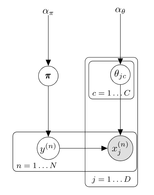
When using a uniform prior $\alpha_\theta=1$, this equation is called Laplace smoothing or add-one smoothing. $\alpha$ intuitively represents a "pseudocount" $\alpha_\theta$ of features $x_{jc}$ . For document classification it simply corresponds to giving an initial non zero count to all words, which avoids the problem of having a test document $x^{(t)}$ with $p(y=c\vert x^{(t)})=0$ if it contains a single word $x_{j}^*$ that has never been seen in a training document with label $c$. $\alpha=1$ is a common choice in examples although smaller often work better .
![]() Side Notes :
Side Notes :
The "Naive" comes from the conditional independence of features given the label. The "Bayes" part of the name comes from the use of Bayes theorem to use a generative model, but it is not a Bayesian method as it does not require marginalizing over all parameters.
If we estimated the Multinomial Naive Bayes using Maximum A Posteriori Estimate (MAP) instead of MSE or the Bayesian way, we would predict using the mode of the posterior (instead of the mean in the Bayesian case) $\hat\theta_{jc}=\frac{N_{jc} + \alpha - 1}{N_c + (\alpha -1)D}$ (similarly for $\pmb\pi$). This means that Laplace smoothing could also be interpreted as using MAP with a non uniform prior $\text{Dir}(\pmb\theta; \pmb{2})$. But when using a uniform Dirichlet prior MAP coincides with the MSE.
Gaussian Naive Bayes is equivalent to Quadratic Discriminant Analysis when each covariance matrix $\Sigma_c$ is diagonal.
Discrete Naive Bayes and Logistic Regression are a "generative-discriminative pair" as they both take the same form (linear in log probabilities) but estimate parameters differently. For example, in the binary case, Naive Bayes predicts the class with the largest probability. I.e. it predicts $C_1$ if $\log \frac{p(C_1 \vert \pmb{x})}{p(C_2 \vert \pmb{x})} = \log \frac{p(C_1 \vert \pmb{x})}{1-p(C_1 \vert \pmb{x})} > 0$. We have seen that discrete Naive Bayes is linear in the log space, so we can rewrite the equation as $\log \frac{p(C_1 \vert \pmb{x})}{1-p(C_1 \vert \pmb{x})} = 2 \log p(C_1 \vert \pmb{x}) - 1 = 2 \left( b + \mathbf{w}^T_c \mathbf{x} \right) - 1 = b' + \mathbf{w'}^T_c \mathbf{x} > 0$. This linear regression on the log odds ratio is exactly the form of Logistic Regression (the usual equation is recovered by solving $\log \frac{p}{1-p} = b + \mathbf{w'}^T \mathbf{x}$). The same can be shown for Multinomial Naive Bayes and Multinomial Logistic Regression.
For document classification, it is common to replace raw counts in Multinomial Naive Bayes with tf-idf weights.
![]() Resources : See section 3.5 of K. Murphy's book for all the derivation steps and examples.
Resources : See section 3.5 of K. Murphy's book for all the derivation steps and examples.