Reinforcement learning
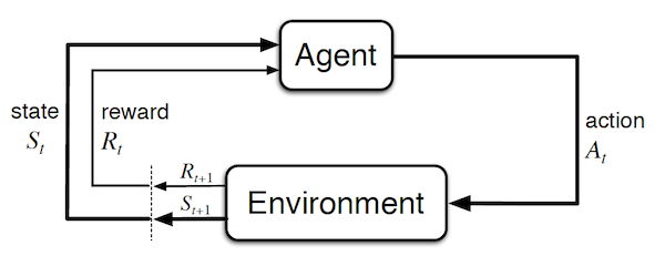
In Reinforcement Learning (RL), the sequential decision-making algorithm (an agent) interacts with an environment it is uncertain about. The agent learns to map situations to actions to maximize a long term reward. During training, the action it chooses are evaluated rather than instructed.
![]() Example: Games can very naturally be framed in a RL framework. For example, when playing tennis you are not told how good every movement you make is, but you are given a certain reward if you win the whole game.
Example: Games can very naturally be framed in a RL framework. For example, when playing tennis you are not told how good every movement you make is, but you are given a certain reward if you win the whole game.
![]() Side Notes: Games could also be framed in a supervised problem. The training set would consist in many different states of the environment and the optimal action to take in each of those. Creating such a dataset is not possible for most applications as it requires to enumerate the exponential number of states and to know the associated best action (e.g. exact rotation of all your joints when you play tennis). Note that during supervised training, the feedback indicates the correct action independently to the chosen action. The RL framework is a lot more natural as the agent is trained by playing the game. Importantly, the agent interacts with the environment such that the states that it will visit depend on previous actions. So it is a chicken-egg problem where it will unlikely reach good states before being trained, but it has to reach good states to get reward and train effectively. This leads to training curves that start with very long plateaus of low reward until it reaches a good state (somewhat by chance) and then learn quickly. In contrast, supervised methods have very steep loss curves at the start.
Side Notes: Games could also be framed in a supervised problem. The training set would consist in many different states of the environment and the optimal action to take in each of those. Creating such a dataset is not possible for most applications as it requires to enumerate the exponential number of states and to know the associated best action (e.g. exact rotation of all your joints when you play tennis). Note that during supervised training, the feedback indicates the correct action independently to the chosen action. The RL framework is a lot more natural as the agent is trained by playing the game. Importantly, the agent interacts with the environment such that the states that it will visit depend on previous actions. So it is a chicken-egg problem where it will unlikely reach good states before being trained, but it has to reach good states to get reward and train effectively. This leads to training curves that start with very long plateaus of low reward until it reaches a good state (somewhat by chance) and then learn quickly. In contrast, supervised methods have very steep loss curves at the start.
![]() Resources : The link and differences between supervised and RL is described in details by A. Barto and T. Dietterich.
Resources : The link and differences between supervised and RL is described in details by A. Barto and T. Dietterich.
In RL, future states depend on current actions, thus requiring to model indirect consequences of actions and planning. Furthermore, the agent often has to take actions in real-time while planning for the future. All of the above makes it very similar to how humans learn, and is thus widely used in psychology and neuroscience.
![]() Resources : All this section on RL is highly influenced by Sutton and Barto's introductory book.
Resources : All this section on RL is highly influenced by Sutton and Barto's introductory book.
Exploration vs Exploitation
A fundamental trade-off in RL is how to balance exploration and exploitation. Indeed, we often assume that the agent has to maximize its reward over all episodes. As it often lacks knowledge about the environment, it has to decide between taking the action it currently thinks is the best, and taking new actions to learn about how good these are (which might bring higher return in the long run).
![]() Example: Lets consider a simplified version of RL - Multi-armed Bandits - to illustrate this concept (example and plots from Sutton and Barto):
Example: Lets consider a simplified version of RL - Multi-armed Bandits - to illustrate this concept (example and plots from Sutton and Barto):
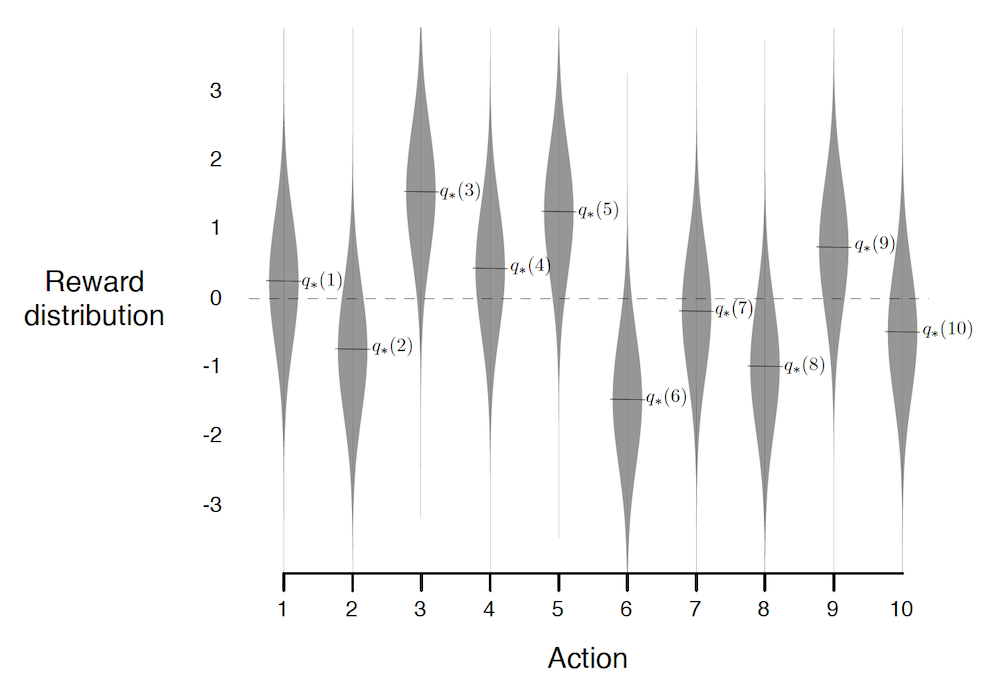
Let's assume that you go in a very generous casino. I.e. an utopic casino in which you can make money in the long run (spoiler alert: this doesn't exist, and in real-life casinos the best action is always to leave ![]() ). This casino contains 10-slot machines, each of these give a certain reward $r$ when the agent decides to play on them. The agent can stay the whole day in this casino and wants to maximize its profit.
). This casino contains 10-slot machines, each of these give a certain reward $r$ when the agent decides to play on them. The agent can stay the whole day in this casino and wants to maximize its profit.
Although the agent doesn't know it, the rewards are sampled as $r \sim \mathcal{N}(\mu_a, 1)$, and each of the 10 machines have a fixed $\mu_a$ which were sampled from $\mathcal{N}(0, 1)$ when building the casino. The actual reward distributions are the following (where $q_{*}(a)$ denote the expected return when choosing slot $a$):
A good agent would try to estimate $Q_t(a) = q_{*}(a)$, where the subscript $t$ indicates that the estimate depends on the time (the more the agent plays the better the estimates should be). The most natural estimate $Q_t(a)$ is to average over all rewards when taking action $a$. At every time step $t$ there's at least one action $\hat{a}=\arg\max_a Q_t(a)$ which the agent believes maximizes $q_{*}(a)$. Taking the greedy action $\hat{a}$ exploits your current beliefs of the environment. This might not always be the "best action", indeed if $\hat{a} \neq a^{*}$ then the agents estimates of the environment are wrong and it would be Better to take a non greedy action $a \neq \hat{a}$ and learn about the environment (supposing it will still play many times). Such actions explore the environment to improve estimates.
During exploration, the reward is often lower in the short run, but higher in the long run because once you discovered better actions you can exploit them many times. Whether to explore or exploit is a complex problem that depends on your current estimates, uncertainties, and the number of remaining steps.
Here are a few possible exploration mechanisms:
- $\pmb{\epsilon}\mathbf{-greedy}$: take the greedy action with probability $1-(\epsilon-\frac{\epsilon}{10})$ and all other actions with probability $\frac{\epsilon}{10}$.
- *Upper-Confidence Bound ** (UCB): $\epsilon\text{-greedy}$ forces the non greedy actions to be tried uniformly. It seems natural to prefer actions that are nearly greedy or particularly uncertain. This can be done by adding a term that measures the variance of the estimate of $Q_t(a)$. Such a term should be inversely proportional to the number of times we have seen an action $N_t(a)$. We use $\frac{\log t}{N_t(a)}$ in order to force the model to take an action $a$ if it has not been taken in a long time (i.e.* if $t$ increases but not $N_t(a)$ then $\frac{\log t}{N_t(a)}$ increases). The logarithm is used in order have less exploration over time but still an infinite amount:
Optimistic Initial Values: gives a highly optimistic $Q_1(a), \ \forall a$ (e.g. $Q_1(a)=5$ in our example, which is a lot larger than $q_{*}(a)$). This ensures that all actions will be at least sampled a few times before following the greedy policy. Note that this permanently biases the action-value estimates when estimating $Q_t(a)$ through averages (although the biases decreases).
Gradient Bandit Algorithms: An other natural way of choosing the best action would be to keep a numerical preference for each action $H_t(a)$. And sample more often actions with larger preference. I.e. sample from $\pi_t := \text{softmax}(H_t)$, where $\pi_t(a)$ denotes the probability of taking action $a$ at time $t$. The preference can then be learned via stochastic gradient ascent, by increasing $H_t(A_t)$ if the reward due to the current action $A_t$ is larger than the current average reward $\bar{R}_t$ (decreasing $H_t(A_t)$ if not). The non selected actions $a \neq A_t$ are moved in the opposite direction. Formally:
By running all the different strategies for different hyperparameters and averaging over 1000 decisions, we get:
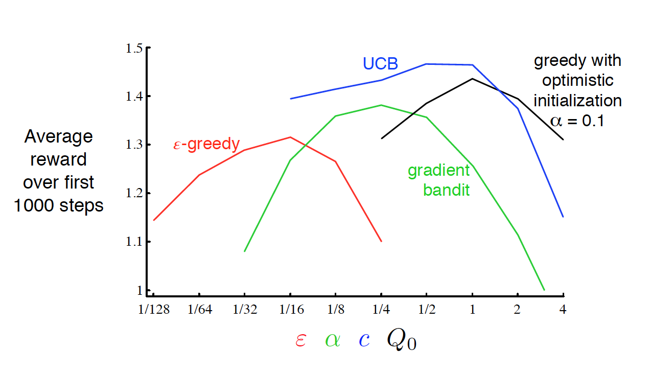
We see that UCB performs best in this case, and is the most robust with regards to its hyper-parameter $c$. Although UCB tends to work well, this will not always be the case (No Free Lunch Theorem again).
![]() Side Notes:
Side Notes:
- In non-stationary environments (I.e. the reward probabilities are changing over time), it is important to always explore as the optimal action might change over time. In such environment, it is better to use exponentially decaying weighted average for $Q_t(a)$. I.e. give more importance to later samples.
- The multi-armed bandits problem, is a simplification of RL as future states and actions are independent of the current action.
- We will see other ways of maintaining exploration in future sections.
Markov Decision Process
Markov Decision Processes (MDPs) are a mathematical idealized form of the RL problem that suppose that states follow the Markov Property. I.e. that future states are conditionally independent of past ones given the present state: $S_{t+1} \perp \{S_{i}\}_{i=1}^{t-1} \vert S_t$.
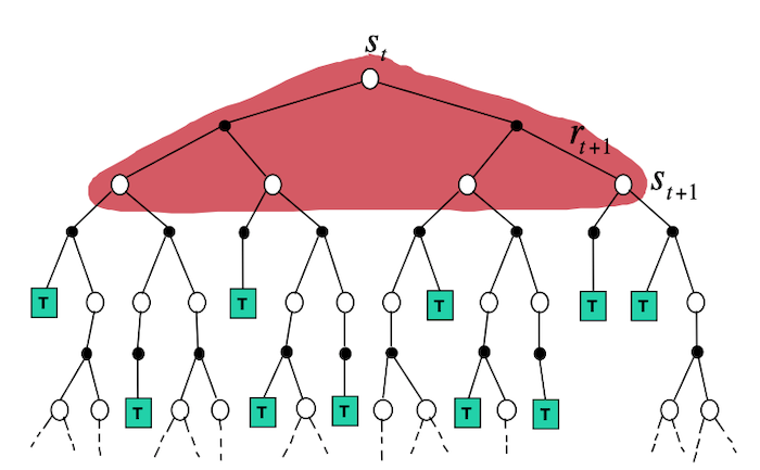
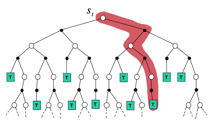
Before diving into the details, it is useful to visualize how simple a MDP is (image taken from Sutton and Barto):
Important concepts:
- Agent: learner and decision maker. This corresponds to the controller in classical control theory.
- Environment: everything outside of the agent. I.e. what it interacts with. It corresponds to the plant in classical control theory. Note that in the case of a human / robot, the body should be considered as the environment rather than as the agent because it cannot be modified arbitrarily (the boundary is defined by the lack of possible control rather than lack of knowledge).
- Time step t: discrete time at which the agent and environment interact. Note that it doesn't have to correspond to fix real-time intervals. Furthermore, it can be extended to the continuous setting.
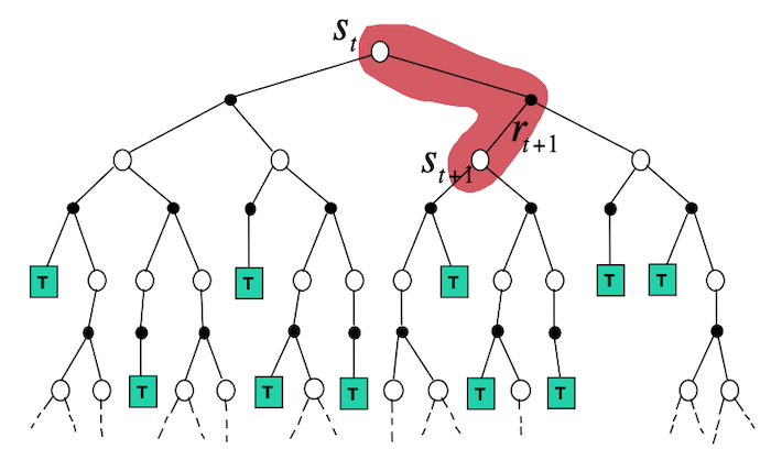
- State $S_t = s \in \mathcal{S}$ : information available to the agent about the environment.
- Action $A_t=a \in \mathcal{A}$ : action that the agent decides to take. It corresponds to the control signal in classical control theory.
- Reward $R_{t+1} = r \in \mathcal{R} \subset \mathbb{R}$: a value which is returned at each step by a (deterministic or stochastic) reward signal function depending on the previous $S_t$ and $A_t$. Intuitively, the reward corresponds to current (short term) pain / pleasure that the agent is feeling. Although the reward is computed inside the agent / brain, we consider them to be external (given by the environment) as they cannot be modified arbitrarily by the agent. The reward signal we choose should truly represent what we want to accomplish , not how to accomplish it (such prior knowledge can be added in the initial policy or value function). For example, in chess, the agent should only be rewarded if it actually wins the game. Giving a reward for achieving subgoals (e.g. taking out an opponent's piece) could result in reward hacking (i.e. the agent might found a way to achieve large rewards without winning).
- Return $G_t := \sum_{\tau=1}^{T-t} \gamma^{\tau-1} R_{t+\tau} \text{, with } \gamma \in [0,1[$: the expected discounted cumulative reward, which has to be maximized by the agent. Note that the discounting factor $\gamma$, has a two-fold use. First and foremost, it enables to have a finite $G_t$ even for continuing tasks $T=\infty$ (opposite of episodic tasks) assuming that $R_t$ is bounded $\forall t$. It also enables to encode the preference for rewards in the near future, and is a parameter that can be tuned to select the "far-sightedness" of your agent ("myopic" agent with $\gamma=0$, "far-sighted" as $\gamma \to 1$). Importantly, the return can be defined in a recursive manner :
- The dynamics of the MDP: $p(s', r\vert s, a) := P(S_{t+1}=s', R_{t+1}=r \vert S_t=s, A_t=a)$. In a MDP, this probability completely characterizes the network dynamics due to the Markov property. Some useful functions that can be derived from it are:
- State-transition probabilities
- Expected rewards for state-actions pairs:
- Expected rewards for state-actions-next state triplets:
- Policy $\pi(a\vert s)$: a mapping from states to probabilities over actions. Intuitively, it corresponds to a "behavioral function". Often called stimulus-response in psychology.
- State-value function for policy $\pi$, $v_\pi(s)$: expected return for an agent that follows a policy $\pi$ and starts in state $s$. Intuitively, it corresponds to how good it is to be in a certain state $s$ (long term). This function is not given by the environment but is often predicted by the agent. Similar to the return, the value function can also be defined recursively, by the very important Bellman equation :
- Action-value function (Q function) for policy $\pi$, $q_\pi(s,a)$: expected total reward and agent can get starting from a state $s$. Intuitively, it corresponds to how good it is to be in a certain state $s$ and take specific action $a$ (long term). A Bellman equation can be derived in a similar way to the value function:
- Model of the environment: an internal model in the agent to predict the dynamic of the environment (e.g. probability of getting a certain reward or getting in a certain state for each action). This is only used by some RL agents for planning.
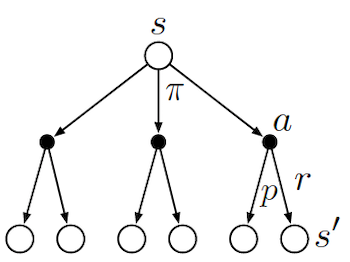
To schematically represents what different algorithms do, it is useful to look at Backup Diagrams. These are trees that are constructed by unrolling all the possible actions and states. White nodes represent a state, from which the agent will follow its policy to select one possible action (black node). The environment will then sample through the dynamics to bring the agent to a new state. Green nodes will be used to denote terminal nodes, and the path taken by the algorithm will be shown in red. Unlike transition graphs, state nodes are not unique (e.g. states can be their own successors). Example:
![]() Side Notes : We usually assume that we have a finite MDP. I.e. that $\mathcal{R},\mathcal{A},\mathcal{S}$ are finite. Dealing with continuous state and actions pairs requires approximations. One possible way of converting a continuous problem to a finite one, is to discretized the state and actions space.
Side Notes : We usually assume that we have a finite MDP. I.e. that $\mathcal{R},\mathcal{A},\mathcal{S}$ are finite. Dealing with continuous state and actions pairs requires approximations. One possible way of converting a continuous problem to a finite one, is to discretized the state and actions space.
In the following sections, we will :
- see how to solve the RL MDP problem exactly through a non linear set of equations or dynamic programing
- approximate the solution by bypassing the need of knowing the dynamics of the system.
- model the dynamics of the system to enable the use of exact methods.
Bellman Optimality Equations
Solving the RL tasks, consists in finding a good policy. A policy $\pi'$ is defined to be better than $\pi \iff v_{\pi'}(s) \geq v_{\pi}(s), \ \forall s \in \mathcal{S}$. The optimal policy $\pi_{*}$ has an associated state optimal value-function and optimal action-value function:
\[v_*(s)=v_{\pi_*}(s):= \max_\pi v_\pi(s)\] \[\begin{aligned} q_*(s,a) &:= q_{\pi_*}(s,a) \\ &= \max_\pi q_\pi(s, a) \\ &= \mathbb{E}[R_{t+1} + \gamma v_*(S_{t+1}) \vert S_{t}=s, A_{t}=a] \end{aligned}\]A special recursive update (the Bellman optimality equations) can be written for the optimal functions $v_{*}$, $q_{*}$ by taking the best action at each step instead of marginalizing:
\[\begin{aligned} v_*(s) &= \max_a q_{\pi_*}(s, a) \\ &= \max_a \mathbb{E}[R_{t+1} + \gamma v_*(S_{t+1}) \vert S_{t}=s, A_{t}=a] \\ &= \max_a \sum_{s'} \sum_r p(s', r \vert s, a) \left[r + \gamma v_*(s') \right] \end{aligned}\] \[\begin{aligned} q_*(s,a) &= \mathbb{E}[R_{t+1} + \gamma \max_{a'} q_*(S_{t+1}, a') \vert S_{t}=s, A_{t}=a] \\ &= \sum_{s'} \sum_{r} p(s', r \vert s, a) \left[r + \gamma \max_{a'} q_*(s', a')\right] \end{aligned}\]The optimal Bellman equations are a set of equations ($\vert \mathcal{S} \vert$ equations and unknowns) with a unique solution. But these equations are now non-linear (due to the max). If the dynamics of the environment were known, you could solve the non-linear system of equation to get $v_{*}$, and follow $\pi_{*}$ by greedily choosing the action that maximizes the expected $v_{*}$. By solving for $q_{*}$, you would simply chose the action $a$ that maximizes $q_{*}(s,a)$, which doesn't require to know anything about the system dynamics.
In practice, the optimal Bellman equations can rarely be solved due to three major problems:
- They require the dynamics of the environment which is rarely known.
- They require large computational resources (memory and computation) to solve as the number of states $\vert \mathcal{S} \vert$ might be huge (or infinite). This is nearly always an issue.
- The Markov Property.
Practical RL algorithms thus settle for approximating the optimal Bellman equations. Usually they parametrize functions and focus mostly on states that will be frequently encountered to make the computations possible.
Dynamic Programming
Overview
-
 Intuition :
- Use dynamic programming as every step only depends on the previous step due to the MDP assumption.
- derives update rules for $v_\pi$ or $q_\pi$ from the Bellman optimality equations to give rise to iterative methods that solve exactly the optimal control problem of finding $\pi_{*}$
-
 Practical:
- DP algorithms are guaranteed to find the optimal policy in polynomial time with respect to $\vert \mathcal{S} \vert$ and \(\vert \mathcal{A} \vert\), even-though the number of possible deterministic policies is $\vert \mathcal{A} \vert ^ {\vert \mathcal{S} \vert}$. This exponential speedup comes from the MDP assumption.
- In practice, DP algorithm converge much faster than the theoretical worst case scenario.
-
 Advantage :
- Exact solution.
-
 Disadvantage :
- Requires the dynamics of the environment.
- Requires large computational resources as $\vert \mathcal{S} \vert$ is usually huge.
- Requires $\infty$ number of iterations to find the exact solution.
- Strongly dependent on the MDP assumption.
- Backup Diagram from David Silver's slides:
![]() Side Notes: DP algorithms use the Bellman equations to update estimates based on other estimates (typically the value function at the next state). This general idea is called Bootstrapping.
Side Notes: DP algorithms use the Bellman equations to update estimates based on other estimates (typically the value function at the next state). This general idea is called Bootstrapping.
Policy Iteration
The high-level idea is to iteratively: evaluate $v_\pi$ for the current policy $\pi$ (policy evaluation 1), use $v_\pi$ to improve $\pi'$ (policy improvement 1), evaluate $v_{\pi'}$ (policy evaluation 2)… Thus obtaining a sequence of strictly monotonically improving policies and value functions (except when converged to $\pi_{*}$). As a finite MDP has only a finite number of possible policies, this is guaranteed to converge in a finite number of steps. This idea is often visualized using a 1d example taken from Sutton and Barto):
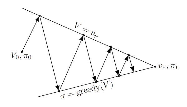
This simplified diagram shows that although the policy improvement and policy evaluation "pull in opposite directions", the 2 processes still converge to find a single joint solution. Almost all RL algorithms can be described using 2 interacting processes (the prediction task for approximating a value, and the control task for improving the policy), which are often called Generalized Policy Iteration (GPI).
In python pseudo-code:
def policy_iteration(environment):
    # v initialized arbitrarily for all states except V(terminal)=0
    v, pi = initialize()
    is_converged = False
    while not is_converged:
        v = policy_evaluation(pi, environment, v)
        pi, is_converged = policy_improvement(v, environment, pi)
    return pi
Policy Evaluation
The first step is to evaluate $v_\pi$ for a given $\pi$. This can be done by solving the Bellman equation :
\[v_\pi(s) = \sum_{a} \pi(a \vert s) \sum_{s'} \sum_r p(s', r\vert s, a) \left[ r + \gamma v_\pi(s') \right]\]Solving the equation can be done by either:
Linear System: This is a set of linear equations ($\vert \mathcal{S} \vert$ equations and unknowns) with a unique solution (if $\gamma <1$ or if it is an episodic task). Note that we would have to solve for these equations at every step of the policy iteration and $\vert \mathcal{S} \vert$ is often very large. Assuming a deterministic policy and reward, this would take $O(\vert \mathcal{S} \vert^3)$ operations to solve.
Iterative method: Modify the Bellman equation to become an iterative method that is guaranteed to converge when $k\to \infty$ if $v_\pi$ exists. This is done by realizing that $v_\pi$ is a fixed point of:
![]() Side Notes : In the iterative method, we would have to keep to keep 2 arrays $v_k(s)$ and $v_{k+1}(s)$. At each iteration $k$ we would update $v_{k+1}(s)$ by looping through all states. Importantly, the algorithm also converges to $v_\pi(s)$ if we keep in memory a single array that would be updated "in-place" (often converges faster as it updates the value for some states using the latest available values). The order of state updates has a significant influence on the convergence in the "in-place" case .
Side Notes : In the iterative method, we would have to keep to keep 2 arrays $v_k(s)$ and $v_{k+1}(s)$. At each iteration $k$ we would update $v_{k+1}(s)$ by looping through all states. Importantly, the algorithm also converges to $v_\pi(s)$ if we keep in memory a single array that would be updated "in-place" (often converges faster as it updates the value for some states using the latest available values). The order of state updates has a significant influence on the convergence in the "in-place" case .
We solve for an approximation $V \approx v_\pi$ by halting the algorithm when the change for every state is "small".
In python pseudo-code:
def q(s, a, v, environment, gamma):
    """Computes the action-value function `q` for a given state and action."""
    dynamics, states, actions, rewards = environment
    return sum(dynamics(s_p,r,s,a) * (r + gamma * v(s_p))
               for s_p in states
               for r in rewards)

def policy_evaluation(pi, environment, v_init, threshold=..., gamma=...):
    dynamics, states, actions, rewards = environment
    V = v_init # don't restart from scratch policy evaluation
    delta = 0
    while delta < threshold :
        delta = 0
        for s in states:
            v = V(s)
            # Bellman update
            V(s) = sum(pi(a, s) * q(a,s, V, environment, gamma) for s_p in states)
            # stop when change for any state is small
            delta = max(delta, abs(v-V(s)))
    return v
Policy Improvement
Now that we have an (estimate of) $v_\pi$ which says how good it is to be in $s$ when following $\pi$, we want to know how to change the policy to yield a higher return.
We have previously defined a policy $\pi'$ to be better than $\pi$ if $v_{\pi'}(s) > v_{\pi}(s), \forall s$. One simple way of improving the current policy $\pi$ would thus be to use a $\pi'$ which is identical to $\pi$ at each state besides one $s_{update}$ for which it will take a better action. Let's assume that we have a deterministic policy $\pi$ that we follow at every step besides one step when in $s_{update}$ at which we follow the new $\pi'$ (and continue with $\pi$). By construction :
\[q_\pi(s, {\pi'}(s)) = v_\pi(s), \forall s \in \mathcal{S} \setminus \{s_{update}\}\] \[q_\pi(s_{update}, {\pi'}(s_{update})) > v_\pi(s_{update})\]Then it can be proved that (Policy Improvement Theorem) :
\[v_{\pi'}(s) \geq v_\pi(s), \forall s \in \mathcal{S} \setminus \{s_{update}\}\] \[v_{\pi'}(s_{update}) > v_\pi(s_{update})\]I.e. if such policy $\pi'$ can be constructed, then it is a better than $\pi$.
The same holds if we extend the update to all actions and all states and stochastic policies. The general policy improvement algorithm is thus :
\[\begin{aligned} \pi'(s) &= arg\max_a q_\pi(s,a) \\ &= arg\max_a \sum_{s'} \sum_r p(s', r\vert s, a) \left[ r + \gamma v_\pi(s') \right] \end{aligned}\]$\pi'$ is always going to be better than $\pi$ except if $\pi=\pi_{*}$, in which case the update equations would turn into the Bellman optimality equation.
In python pseudo-code:
def policy_improvement(v, environment, pi):
    dynamics, states, actions, rewards = environment
    is_converged = True
    for s in states:
        old_action = pi(s)
        # q defined in `policy_evaluation` pseudo-code
        pi(s) = argmax(q(s,a, v, environment, gamma) for a in actions)
        if old_action != pi(s):
            is_converged = False
    return pi, is_converged
![]() Practical : Assuming a deterministic reward, this would take $O(\vert \mathcal{S} \vert^2 \vert \mathcal{A} \vert)$ operations to solve. Each iteration of the policy iteration algorithm thus takes $O(\vert \mathcal{S} \vert^2 (\vert \mathcal{S} \vert + \vert \mathcal{A} \vert))$ for a deterministic policy and reward signal, if we solve the linear system of equations for the policy evaluation step.
Practical : Assuming a deterministic reward, this would take $O(\vert \mathcal{S} \vert^2 \vert \mathcal{A} \vert)$ operations to solve. Each iteration of the policy iteration algorithm thus takes $O(\vert \mathcal{S} \vert^2 (\vert \mathcal{S} \vert + \vert \mathcal{A} \vert))$ for a deterministic policy and reward signal, if we solve the linear system of equations for the policy evaluation step.
Value Iteration
In policy iteration, the bottleneck is the policy evaluation which requires multiple loops over the state space (convergence only for an infinite number of loops). Importantly, the same convergence guarantees as with policy iteration hold when doing a single policy evaluation step. Policy iteration with a single evaluation step, is called value iteration and can be written as a simple update step that combines the truncated policy evaluation and the policy improvement steps:
\[v_{k+1}(s) = \max_{a} \sum_{s'} \sum_r p(s', r\vert s, a) \left[ r + \gamma v_{k}(s') \right], \ \forall s \in \mathcal{S}\]This is guaranteed to converge for arbitrary $v_0$ if $v_*$ exists. Value iteration corresponds to the update rule derived from the Bellman optimality equation . The formula, is very similar to policy evaluation, but it maximizes instead of marginalizing over actions.
Like policy evaluation, value iteration needs an infinite number of steps to converge to $v_*$. In practice we stop whenever the change for all actions is small.
In python pseudo-code:
def value_to_policy(v, environment, gamma):
    """Makes a deterministic policy from a value function."""
    dynamics, states, actions, rewards = environment
    pi = dict()
    for s in states:
        # q defined in `policy_evaluation` pseudo-code
        pi(s) = argmax(q(s,a, v, environment, gamma) for a in actions)
    return pi

def value_iteration(environment, threshold=..., gamma=...):
    dynamics, states, actions, rewards = environment
    # v initialized arbitrarily for all states except V(terminal)=0
    V = initialize()
    delta = threshold + 1 # force at least 1 pass
    while delta < threshold :
        delta = 0
        for s in states:
            v = V(s)
            # Bellman optimal update
            # q defined in `policy_evaluation` pseudo-code
            V(s) = max(q(s, a, v, environment, gamma) for a in actions)
            # stop when change for any state is small
            delta = max(delta, abs(v-V(s)))
    pi = value_to_policy(v, environment, gamma)
    return pi
![]() Practical : Faster convergence is often achieved by doing a couple of policy evaluation sweeps (instead of a single one in the value iteration case) between each policy improvement. The entire class of truncated policy iteration converges. Truncated policy iteration can be schematically seen as using the modified generalized policy iteration diagram:
Practical : Faster convergence is often achieved by doing a couple of policy evaluation sweeps (instead of a single one in the value iteration case) between each policy improvement. The entire class of truncated policy iteration converges. Truncated policy iteration can be schematically seen as using the modified generalized policy iteration diagram:
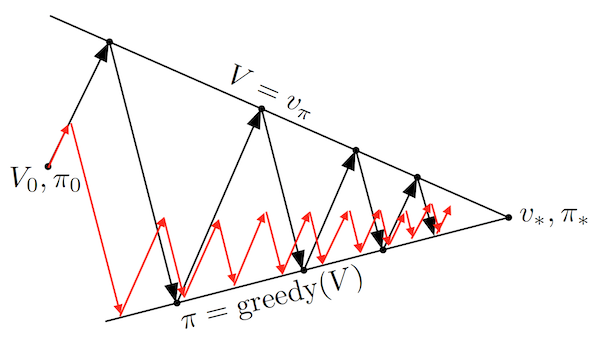
As seen above, truncated policy iteration uses only approximate value functions. This usually increases the number of required policy evaluation and iteration steps, but greatly decreases the number of steps per policy iteration making the overall algorithm usually quicker. Assuming a deterministic policy and reward signal, each iteration for the value iteration takes $O(\vert \mathcal{S} \vert^2 \vert \mathcal{A} \vert)$ which is less than exact (solving the linear system) policy iteration $O(\vert \mathcal{S} \vert^2 (\vert \mathcal{S} \vert + \vert \mathcal{A} \vert))$.
Asynchronous Dynamic Programming
A drawback of DP algorithms, is that they require to loop over all states for a single sweep. Asynchronous DP algorithms are in-place iterative methods that update the value of each state in any order. Such algorithms are still guaranteed to converge as long as it can't ignore any state after some points (for the episodic case it is also easy to avoid the few orderings that do not converge).
By carefully selecting the states to update, we can often improve the convergence rate. Furthermore, asynchronous DP enables to update the value of the states as the agent visits them. This is very useful in practice, and focuses the computations on the most relevant states.
![]() Practical : Asynchronous DP are usually preferred for problems with large state-spaces
Practical : Asynchronous DP are usually preferred for problems with large state-spaces
Non DP Exact Methods
Although DP algorithms are the most used for finding exact solution of the Bellman optimality equations, other methods can have better worst-case convergence guarantees. Linear Programming (LP) is one of those methods. Indeed, the Bellman optimality equations can be written as a linear program. Let $B$ be the Bellman operator (i.e. $v_{k+1} = B(v_k)$), and $\pmb{\mu_0}$ is a probability distribution over states, then:
\[\begin{array}{ccc} v_* = & arg\min_{v} & \pmb{\mu}_0^T \mathbf{v} \\ & \text{s.t.} & \mathbf{v} \geq B(\mathbf{v}) \\ \end{array}\]Indeed, if $v \geq B(v)$ then $B(v) \geq B(B(v))$ due to the monotonicity of the Bellman operator. By repeated applications we must have that $v \geq B(v) \geq B(B(v)) \geq B^3(v) \geq \ldots \geq B^{\infty}(v) = v_{*}$. Any solution of the LP must satisfy $v \geq B(v)$ and must thus be $v_{*}$. Then the objective function $\pmb{\mu}_0^T \mathbf{v}$ is the expected cumulative reward when beginning at a state drawn from $\pmb{\mu}_0$. By substituting for the Bellman operator $B$:
\[\begin{array}{ccc} v_* = & arg\min_{v} & \sum_s \mu_0(s) v(s) \\ & \text{s.t.} & v(s) \geq \sum_{s'} \sum_{r} p(s', r \vert s , a) \left[r + \gamma v(s') \right]\\ & & \forall s \in \mathcal{s}, \ \forall a \in \mathcal{A} \end{array}\]Using the dual form of the LP program, the equation above can be rewritten as :
\[\begin{aligned} \max_\lambda & \sum_s \sum_a \sum_{s'} \sum_r \lambda(s,a) p(s', r \vert s , a) r\\ \text{s.t.} & \sum_a \lambda(s',a) = \mu_0(s') + \gamma \sum_s \sum_a p(s'|s,a) \lambda(s,a) \\ & \lambda(s,a) \geq 0 \\ & \forall s' \in \mathcal{s} \end{aligned}\]The constraints in the dual LP ensure that :
\[\lambda(s,a) = \sum_{t=0}^\infty \gamma^t p(S_t=s, A_t=a)\]I.e. they are the discounted state-action counts. While the dual objective maximizes the expected discounted return. The optimal policy can is :
$\pi_*(s)=max_a \mu(s,a)$
![]() Practical: Linear programming is sometimes better than DP for small number of states, but it does not scale well.
Practical: Linear programming is sometimes better than DP for small number of states, but it does not scale well.
Although LP are rarely useful, they provide connections to a number of other methods that have been used to find approximate large-scale MDP solutions.
Monte Carlo GPI
Overview
-
Intuition :
- Approximates Generalized Policy Iteration by estimating the expectations through sampling rather than computing them.
- The idea is to estimate the value function by following a policy and averaging returns over multiple episodes, then updating the value function at every visited state.
-
Advantage :
- Can learn from experience, without explicit knowledge of the dynamics.
- Unbiased
- Less harmed by MDP violation because they do not bootstrap.
- Not very sensitive to initialization
-
Disadvantage :
- High variance because depends on many random actions, transitions, rewards
- Have to wait until end of episode to update.
- Only works for episodic tasks.
- Slow convergence.
- Suffer if lack of exploration.
- Backup Diagram
As mentioned previously, the dynamics of the environment are rarely known. In such cases we cannot use DP. Monte Carlo (MC) methods bypass this lack of knowledge by estimating the expected return from experience (i.e. sampling of the unknown dynamics).
MC methods are very similar to the previously discussed Generalized Policy Iteration(GPI). The main differences being:
They learn the value-function by sampling from the MDP (experience) rather than computing these values using the dynamics of the MDP.
MC methods do not bootstrap: each value function for each state/action is estimated independently. I.e. they do not update value estimates based on other value estimates.
In DP, given a state-value function, we could look ahead one step to determine a policy. This is not possible anymore due to the lack of knowledge of the dynamics. It is thus crucial to estimate the action value function $q_{*}$ instead of $v_{*}$ in policy evaluation.
Recall that $q_\pi(s) = \mathbb{E}[R_{t+1} + \gamma G_{t+1} \vert S_{t}=s, A_t=a]$. Monte Carlo Estimation approximates this expectations through sampling. I.e. by averaging the returns after every visits of state action pairs $(s,a)$.
Note that pairs $(s,a)$ could be visited multiple times in the same episode. How we treat these visits gives rise to 2 slightly different methods:
- First-visit MC Method: estimate $q_\pi(s,a)$ as the average of the returns following the first visit to $(s,a)$. This has been more studied and is the one I will be using.
- Every-visit MC Method: estimate $q_\pi(s,a)$ as the average of the returns following all visit to $(s,a)$. These are often preferred as they don't require to keep track of which states have been visited.
Both methods converge to $q_\pi(s,a)$ as the number of visits $n \to \infty$. The convergence of the first-visit MC is easier to prove as each return is an i.i.d estimate of $q_\pi(s,a)$. The standard deviation of the estimate drops with $\frac{1}{\sqrt{n}}$.
![]() Side Notes:
Side Notes:
- MC methods can learn from actual experience or simulated one. The former is used when there's no knowledge about the dynamics. The latter is useful when it is possible to generate samples of the environment but infeasible to write it explicitly. For example, it is very easy to simulate a game of blackjack, but computing $p(s',r' \vert s,a)$ as a function of the dealer cards is complicated.
- The return at each state depends on the future action. Due to the training of the policy, the problem becomes non-stationary from the point of view of the earlier states.
- In order to have well defined returns, we will only be considering episodic tasks (i.e. finite $T$)
- The idea is the same as in Bayesian modeling, where we approximated expectations by sampling.
- MC methods do not bootstrap and are thus very useful to compute the value of only a subset of states, by starting many episodes at the state of interests.
On-Policy Monte Carlo GPI
Let's make a simple generalized policy iteration (GPI) algorithm using MC methods. As a reminder, GPI consists in iteratively alternating between evaluation (E) and improvement (I) of the policy, until we reach the optimal policy:
\[\pi _ { 0 } \stackrel { \mathrm { E } } { \longrightarrow } q _ { \pi _ { 0 } } \stackrel { \mathrm { I } } { \longrightarrow } \pi _ { 1 } \stackrel { \mathrm { E } } { \longrightarrow } q _ { \pi _ { 1 } } \stackrel { \mathrm { I } } { \longrightarrow } \pi _ { 2 } \stackrel { \mathrm { E } } { \longrightarrow } \cdots \stackrel { \mathrm { I } } { \longrightarrow } \pi _ { * } \stackrel { \mathrm { E } } { \rightarrow } q _ { * }\]- Generalized Policy Evaluation (prediction). Evaluates the value function $Q \approx q_\pi$ (not $V$ as we do not have the dynamics). Let $F_i(s,a)$ return the time step $t$ at which state-action pair $(s,a)$ is first seen (first-visit MC) in episode $i$ (return $-1$ if never seen), and $G_{t}^{(i)}(\pi)$ be the discounted return from time $t$ of the $i^{th}$ episode when following $\pi$:
- Policy Improvement, make a GLIE (defined below) policy $\pi$ from $Q$. Note that the policy improvement theorem still holds.
Unsurprisingly, MC methods can be shown to converge if they maintain exploration and when the policy evaluation step uses an $\infty$ number of samples. Indeed, these 2 conditions ensure that all expectations are correct as MC sampling methods are unbiased.
Of course using an $\infty$ number of samples is not possible, and we would like to alternate (after every episode) between evaluation and improvement even when evaluation did not converge (similarly value iteration). Although MC methods cannot converge to a suboptimal policy in this case, the fact that it converges to the optimal fixed point has yet to be formally proved.
Maintaining exploration is a major issue. Indeed, if $\pi$ is deterministic then the samples will only improve estimates for one action per state. To ensure convergence we thus need a policy which is Greedy in the Limit with Infinite Exploration (GLIE). I.e. : 1/ All state-action pairs have to be explored infinitely many times; 2/ The policy has to converge to a greedy one. Possible solutions include:
- Exploring Starts: start every episode with a sampled state-action pair from a distribution that is non-zero for all pairs. This ensures that all pairs $(s,a)$ will be visited an infinite number of times as $n \to \infty$. Choosing starting conditions is often not applicable (e.g. most games always start from the same position).
- Non-Zero Stochastic Policy: to ensure that all pairs $(s,a)$ are encountered, use a stochastic policy with a non-zero probability for all actions in each state. $\epsilon\textbf{-greedy}$ is a well known policy, which takes the greedy action with probability $1-(\epsilon+\frac{\epsilon}{\vert \mathcal{A} \vert})$ and assigns a uniform probability of $\frac{\epsilon}{\vert \mathcal{A} \vert}$ to all other actions. To be a GLIE policy, $\epsilon$ has to converge to 0 in the limit (e.g. $\frac{1}{t}$).
In python pseudo-code:
def update_eps_policy(Q, pi, s, actions, eps):
    """Update an epsilon policy for a given state."""
    q_best = -float("inf")
    for a in actions:
        pi[(a, s)] = eps/len(actions)
        q_a = Q[(s, a)]
        if q_a  > q_best:
            q_best = q_a
            a_best = a
    pi[(a_best, s)] = 1 - (eps - (eps/len(actions)))
    return pi

def q_to_eps_pi(Q, eps, actions, states):
    """Creates an epsilon policy from a action value function."""
    pi = defaultdict(lambda x: 0)
    for s in states:
        pi = update_eps_policy(Q, pi, s, actions, eps)
    return pi

def on_policy_mc(game, actions, states, n=..., eps=..., gamma=...):
    """On policy Monte Carlo GPI using first-visit update and epsilon greedy policy."""
    returns = defaultdict(list)
    Q = defaultdict(lambda x: 0)
    for _ in range(n):
        pi = q_to_eps_pi(Q, eps, actions, states)
        T, list_states, list_actions, list_rewards = game(pi)
        G = 0
        for t in range(T-1,-1,-1): # T-1, T-2, ... 0
            r_t, s_t, a_t = list_rewards[t], list_states[t], list_actions[t]
            G = gamma * G + r_t # current return
            if s_t not in list_states[:t]: # if first
                returns[(s_t, a_t)].append(G)
                Q[(s_t, a_t)] = mean(returns[(s_t, a_t)]) # mean over all episodes
    return V
Incremental Implementation
The MC methods can be implemented incrementally. Instead of getting estimates of $q_\pi$ by keeping in memory all $G_t^{(i)}$ to average over those, the average can be computed exactly at each step $n$. Let $m := \sum_i \mathcal{I}[F_i(s,a) \neq -1]$, then:
\[\begin{aligned} Q_{m+1}(s,a) &= \frac{1}{m} \sum_{i:G_{F_i(s,a)}^{(i)}(\pi)\neq -1}^m G_{F_i(s,a)}^{(i)}(\pi)\\ &= \frac{1}{m} \left(G_{F_m(s,a)}^{(m)}(\pi) + \sum_{i:G_{F_i(s,a)}^{(i)}(\pi)\neq -1}^{m-1} G_{F_i(s,a)}^{(i)}(\pi)\right)\\ &= \frac{1}{m} \left(G_{F_m(s,a)}^{(m)}(\pi) + (m-1)\frac{1}{m-1} \sum_{i:G_{F_i(s,a)}^{(i)}(\pi)\neq -1}^{m-1} G_{F_i(s,a)}^{(i)}(\pi)\right)\\ &= \frac{1}{m} \left(G_{F_m(s,a)}^{(m)}(\pi) + (m-1)Q_{m}(s,a) \right) \\ &= Q_{m}(s,a) + \frac{1}{m} \left(G_{F_m(s,a)}^{(m)}(\pi) - (m-1)Q_{m}(s,a) \right) \\ \end{aligned}\]This is of the general form :
\[\textrm{new_estimate}=\textrm{old_estimate} + \alpha_n \cdot (\textrm{target}-\textrm{old_estimate})\]Where the step-size $\alpha_n$ varies as it is $\frac{1}{n}$. In RL, problems are often non-stationary, in which case we would like to give more importance to recent samples. A popular way of achieving this, is by using a constant step-size $\alpha \in ]0,1]$. This gives rise to an exponentially decaying weighted average (also called exponential recency-weighted average in RL). Indeed:
\[\begin{aligned} Q_{m+1}(s,a) &= Q_{m}(s,a) + \alpha \left(G_{F_m(s,a)}^{(m)}(\pi)- Q_{m}(s,a) \right) \\ &= \alpha G_{F_m(s,a)}^{(m)}(\pi) + (1-\alpha)Q_{m}(s,a) \\ &= \alpha G_{F_m(s,a)}^{(m)}(\pi) + (1-\alpha) \left( \alpha G_{F_m(s,a)}^{(m)}(\pi) + (1-\alpha)Q_{m-1}(s,a) \right) \\ &= (1-\alpha)^mQ_1 + \sum_{i=1}^m \alpha (1-\alpha)^{m-i} G_{F_i(s,a)}^{(i)}(\pi) & \text{Recursive Application} \\ \end{aligned}\]![]() Intuition: At every step we update our estimates by taking a small step towards the goal, the direction (sign in 1D) is given by the error $\epsilon = \left(G_{F_m(s,a)}^{(m)}(\pi) - Q_{n}(s,a) \right)$ and the steps size by $\alpha * \vert \epsilon \vert$.
Intuition: At every step we update our estimates by taking a small step towards the goal, the direction (sign in 1D) is given by the error $\epsilon = \left(G_{F_m(s,a)}^{(m)}(\pi) - Q_{n}(s,a) \right)$ and the steps size by $\alpha * \vert \epsilon \vert$.
![]() Side Notes:
Side Notes:
- The weight given the $i^{th}$ return $G_{F_i(s,a)}^{(i)}(\pi)$ is $\alpha(1-\alpha)^{n-i}$, which decreases exponentially as i decreases ($(1-\alpha) \in [0,1[$).
- It is a well weighted average because the sum of the weights can be shown to be 1.
- From stochastic approximation theory we know that we need a Robbins-Monro sequence of $\alpha_n$ for convergence: $\sum_{m=1}^{\infty} \alpha_m = \infty$ (steps large enough to overcome initial conditions / noise) and $\sum_{m=1}^{\infty} \alpha_m^2 < \infty$ (steps small enough to converge). This is the case for $\alpha_m = \frac{1}{m}$ but not for a constant $\alpha$. But in non-stationary environment we actually don't want the algorithm to converge, in order to continue learning.
- For every-visit MC, this can simply be rewritten as the following update step at the end of each episode:
Off-Policy Monte Carlo GPI
In the on-policy case we had to use a hack ($\epsilon \text{-greedy}$ policy) in order to ensure convergence. The previous method thus compromises between ensuring exploration and learning the (nearly) optimal policy. Off-policy methods remove the need of compromise by having 2 different policy.
The behavior policy $b$ is used to collect samples and is a non-zero stochastic policy which ensures convergence by ensuring exploration. The target policy $\pi$ is the policy we are estimating and will be using at test time, it focuses on exploitation. The latter is often a deterministic policy. These methods contrast with on-policy ones, that uses a single policy.
![]() Intuition: The intuition behind off-policy methods is to follow an other policy but to weight the final return in such a way that compensates for the actions taken by $b$. This can be done via Importance Sampling without biasing the final estimate.
Intuition: The intuition behind off-policy methods is to follow an other policy but to weight the final return in such a way that compensates for the actions taken by $b$. This can be done via Importance Sampling without biasing the final estimate.
Given a starting state $S_t$ the probability of all subsequent state-action trajectory $A_t, S_{t+1}, A_{t+1}, \ldots, S_T$ when following $\pi$ is:
\[P(A_t, S_{t+1}, A_{t+1}, \ldots, S_T \vert S_t, A_{t:T-1} \sim \pi) = \prod_{k=t}^{T-1} \pi (A_k \vert S_k) p(S_{k+1} \vert S_k, A_k)\]Note that the dynamics $p(s' \vert s, a)$ are unknown but we only care about the ratio of the state-action trajectory when following $\pi$ and $b$. The importance sampling ratio is:
\[\begin{aligned} w_{t:T-1} &= \frac{P(A_t, S_{t+1}, A_{t+1}, \ldots, S_T \vert S_t, A_{t:T-1} \sim \pi)}{P(A_t, S_{t+1}, A_{t+1}, \ldots, S_T \vert S_t, A_{t:T-1} \sim b) }\\ &= \frac{\prod_{k=t}^{T-1} \pi (A_k \vert S_k) p(S_{k+1} \vert S_k, A_k)}{\prod_{k=t}^{T-1} b (A_k \vert S_k) p(S_{k+1} \vert S_k, A_k)}\\ &= \prod_{k=t}^{T-1} \frac{ \pi (A_k \vert S_k) }{b (A_k \vert S_k)} \end{aligned}\]Note that if we simply average over all returns we would get $\mathbb{E}[G_t \vert S_t=s] = v_b(s)$, to get $v_\pi(s)$ we can use the previously computed importance sampling ratio:
\[\mathbb{E}[w_{t:T-1} G_t \vert S_t=s] = v_\pi(s)\]![]() Side Notes:
Side Notes:
- Off policy methods are more general as on policy methods can be written as off-policy methods with the same behavior and target policy.
- In order to estimate values of $\pi$ using $b$ we require $\pi(a \vert s) \ge 0 \implies b(a\vert s) \ge$ (coverage assumption). I.e. all actions of $\pi$ can be taken by $b$.
- The formula shown above is the ordinary importance sampling, although it is unbiased it can have large variance. Weighted importance sampling is biased (although it is a consistent estimate as the bias decreases with $O(1/n)$) but is usually preferred as the variance is usually dramatically smaller:
- The importance method above treats the returns $G_0$ as a whole, without taking into account the discount factors. For example if $\gamma=1$, then $G_0 = R_1$, we would thus only need the importance sampling ratio $\frac{pi(A_0 \vert S_0)}{b(A_0 \vert S_0)}$, yet we currently use also the 99 other factors $\frac{pi(A_1 \vert S_1)}{b(A_1 \vert S_1)} \ldots \frac{pi(A_{99} \vert S_{99})}{b(A_{99} \vert S_{99})}$ which greatly increases the variance. Discounting-aware importance sampling greatly decreases the variance by taking the discounts into account.
![]() Practical: Off-policy methods are very useful to learn by seeing a human expert or non-learning controller.
Practical: Off-policy methods are very useful to learn by seeing a human expert or non-learning controller.
In python pseudo-code:
def off_policy_mc(Q, game, b, actions, n=..., gamma=...):
    """Off policy Monte Carlo GPI using incremental update and weighted importance sampling."""
    pi = dict()
    returns = defaultdict(list)
    Q = defaultdict(lambda x: random.rand)
    C = defaultdict(lambda x: 0)
    for _ in range(n):
        T, list_states, list_actions, list_rewards = game(b)
        G = 0
        W = 1
        for t in range(T-1,-1,-1): # T-1, T-2, ... 0
            r_t, s_t, a_t = list_rewards[t], list_states[t], list_actions[t]
            G = gamma * G + r_t # current return
            C[(s_t, a_t)] += W
            Q[(s_t, a_t)] += (W/C[(s_t, a_t)])(G-Q[(s_t, a_t)])
            pi[s_t] = argmax(Q[(s_t, a)] for a in actions)
            if a_t != pi(s):
                break
            W /= b[(s_t, a_t)]
    return V
![]() Side Notes: As for on policy, Off policy MC control can also be written in an Incremental manner. The details can be found in chapter 5.6 of Sutton and Barto.
Side Notes: As for on policy, Off policy MC control can also be written in an Incremental manner. The details can be found in chapter 5.6 of Sutton and Barto.
Temporal-Difference Learning
Overview
-
Intuition :
- Modify Monte Carlo methods to update estimates from other estimates without having to wait for a final outcome.
-
Advantage :
- Can learn from experience, without explicit knowledge of the dynamics.
- Can compute the value of only a subset of states.
- On-line learning by updating at every step.
- Works in continuing (non-terminating) environments
- Low variance as only depends on a single random action, transition, reward
- Very effective in Markov environments (exploit the property through bootstrapping)
-
Disadvantage :
- Suffer if Markov property does not hold.
- Suffer if lack of exploration.
- Backup Diagram:
The fundamental idea of temporal-difference (TD) learning is to remove the need of waiting until the end of an episode to get $G_t$ in MC methods, by taking a single step and update using $R_{t+1} + \gamma V(S_{t+1}) \approx G_t$. Note that when the estimates are correct, i.e. $V(S_{t+1}) = v_\pi(S_{t+1})$, then $\mathbb{E}[R_{t+1} + \gamma V(S_{t+1})] = \mathbb{E}[G_t]$.
As we have seen, incremental MC methods for evaluating $V$, can be written as $V_{k+1}(S_t) = V_{k}(S_t) + \alpha \left( G_t - V_{k}(S_t) \right)$. Using bootstrapping, this becomes:
\[V_{k+1}(S_t) = V_{k}(S_t) + \alpha \left( R_{t+1} + \gamma V_k(S_{t+1}) - V_{k}(S_t) \right)\]This important update is called $\textbf{TD(0)}$, as it is a specific case of TD(lambda). The error term that is used to update our estimate, is very important in RL and Neuroscience. It is called the TD Error:
\[\delta_t := R_{t+1} + \gamma V(S_{t+1}) - V(S_t)\]Importantly $\text{TD}(0)$ always converges to $v_\pi$ if $\alpha$ decreases according to the usual stochastic conditions (e.g. $\alpha = \frac{1}{t}$). Although, the theoretical difference in speed of convergence of TD(0) and MC methods is still open, the former often converges faster in practice.
![]() Side Notes:
Side Notes:
- $\delta_t$ is the error in $V(S_t)$ but is only available at time $t+1$.
- The MC error can be written as a sum of TD errors if $V$ is not updated during the episode: $G_t - V(S_t) = \sum_{k=t}^{T-1} \gamma^{k-t} \delta_k$
- Updating the value with the TD error, is called the backup
- the name comes from the fact that you look at the difference between estimates of consecutive time.
- For batch updating (i.e. single batch of data that is processed multiple times and the model is updated after each batch pass), MC and TD(0) do not in general find the same answer. MC methods find the estimate that minimizes the mean-squared error on the training set, while TD(0) finds the maximum likelihood estimate of the Markov Process. For example, suppose we have 2 states $A$, $B$ and a training data $\{(A:0:B:0), (B:1), (B:1), (B:0)\}$. What should $V(A)$ be? There are at least 2 answers that make sense. MC methods would answer $V(A)=0$ because every time $A$ has been seen, it resulted in a reward of $0$. This doesn't take into account the Markov property. Conversely, $TD(0)$ would answer $V(A)=0.5$ because $100\%$ of $A$ transited to $B$. Using the Markov assumption, the rewards should be independent of the past once we are in state $B$. I.e. $V(A)=V(B)=\frac{2}{4}=\frac{1}{2}$.
On-Policy TD GPI (SARSA)
Similarly to MC methods, we need an action-value function $q_\pi$ instead of a state one $v_\pi$ because we do not know the dynamics and thus cannot simply learn the policy from $v_\pi$. Replacing TD estimates in on policy MC GPI, we have:
- Generalized Policy Evaluation (Prediction): this update is done for every transition from a non-terminal state $S_t$ (set $Q(s_{terminal},A_{t+1})=0$):
- Policy Improvement: make a GLIE policy $\pi$ from $Q$. Note that the policy improvement theorem still holds.
![]() Side Notes:
Side Notes:
- The update rule uses the values $(S_t, A_t, R_{t+1}, S_{t+1}, A_{t+1})$, which gave its name.
- As with On policy MC GPI, you have to ensure sufficient exploration which can be done using an $\epsilon\text{-greedy}$ policy.
- As with MC, the algorithm converges to an optimal policy as long as the policy is GLIE.
In python pseudo-code:
def sarsa(game, states, actions, n=..., eps=..., gamma=..., alpha=...):
    """SARSA using epsilon greedy policy."""
    Q = defaultdict(lambda x: 0)
    pi = q_to_eps_pi(Q, eps, actions, states) # defined in on policy MC
    for _ in range(n):
        s_t = game() #initializes the state
        a_t = sample(pi, s_t)
        while s_t not is terminal:
            s_t1, r_t = game(s_t, a_t) # single run
            # compute A_{t+1} for update
            a_t1 = sample(pi, s_t1)
            Q[(s_t, a_t)] += alpha * (r_t + gamma*Q[(s_t1, a_t1)] - Q[(s_t, a_t)])
            pi = update_eps_policy(Q, pi, s_t, actions, eps) # defined in on policy MC
            s_t, a_t = s_t1, a_t1
    return pi
Off Policy TD GPI (Q-Learning)
Just as with off-policy MC, TD can be written as an off-policy algorithm. In this case, the TD error is not computed with respect to the next sample but with respect to the current optimal greedy policy (i.e. the one maximizing the current action-value function $Q$)
- Generalized Policy Evaluation (Prediction):
- Policy Improvement: make a GLIE policy $\pi$ from $Q$.
The algorithm can be proved to converge as long as all state-action pairs continue being updated.
In python pseudo-code:
def q_learning(game, states, actions, n=..., eps=..., gamma=..., alpha=...):
    """Q learning."""
    Q = defaultdict(lambda x: 0)
    pi = q_to_eps_pi(Q, eps, actions, states) # defined in on policy MC
    for _ in range(n):
        s_t = game() # initializes the state
        while s_t not is terminal:
            a_t = sample(pi, s_t)
            s_t1, r_t = game(s_t, a_t) # single run
            a_best = argmax(Q[(s_t1, a)] for a in actions)
            Q[(s_t, a_t)] += alpha * (r_t + gamma*a_best - Q[(s_t, a_t)])
            pi = update_eps_policy(Q, pi, s_t, actions, eps) # defined in on policy MC
            s_t, = s_t1
    return pi