Latent NPFs
Overview
We concluded the previous section by noting two important drawbacks of the CNPF:
The predictive distribution is factorised across target points, and thus can neither account for correlations in the predictive nor (as a result) produce “coherent” samples from the predictive distribution.
The predictive distribution requires specification of a particular parametric form (e.g. Gaussian).
In this section we discuss an alternative parametrisation of \(p_\theta( \mathbf{y}_\mathcal{T} | \mathbf{x}_\mathcal{T}; \mathcal{C})\) that still satisfies our desiredata for NPs, and addresses both of these issues. The main idea is to introduce a latent variable \(\mathbf{z}\) into the definition of the predictive distribution. This leads us to the second major branch of the NPF, which we refer to as the Latent Neural Process Sub-family, or LNPF for short. A graphical representation of the LNPF is given in Fig. 31.
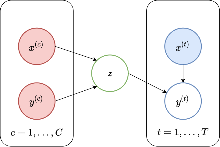
Fig. 31 Probabilistic graphical model for LNPs.
Disclaimer\(\qquad\) (Latent) Neural Processes Family
In this tutorial, we refer use the adjective “Latent” to distinguish the Latent NPF from the Conditional NPF. We then use term “neural process” to refer to both conditional neural processes and latent neural processes. In the literature, however, the term “neural process” is used to refer to “latent neural processes”. As a result the models that we will discuss and call LNP, AttnLNP, and ConvLNP are found in the literature under the abbreviations NP, AttnNP, ConvNP.
To specify this family of models, we must define a few components:
An encoder: \(p_{\theta} \left( \mathbf{z} | \mathcal{C} \right)\), which provides a distribution over the latent variable \(\mathbf{z}\) having observed the context set \(\mathcal{C}\). As with other NPF, the encoder needs to be permutation invariant to correctly treat \(\mathcal{C}\) as a set. A typical example is to first have a deterministic representation \(R\) and then use it to output the mean and (log) standard deviations of a Gaussian distribution over \(\mathbf{z}\).
A decoder: \(p_{\theta} \left( \mathbf{y}_{\mathcal{T}} | \mathbf{x}_{\mathcal{T}}, \mathbf{z} \right)\), which provides predictive distributions conditioned on \(\mathbf{z}\) and a target location \(\mathbf{x}_{\mathcal{T}}\). The decoder will usually be the same as the CNPF, but using a sample of the latent representation \(\mathbf{z}\) and marginalizing them, rather than a deterministic representation.
Putting altogether:
Advanced\(\qquad\)Marginalisation and Factorisation \(\implies\) Consistency
We show that like the CNPF, members of the LNPF also specify consistent stochastic processes conditioned on a fixed context set \(\mathcal{C}\).
(Consistency under permutation) Let \(\mathbf{x}_{\mathcal{T}} = \{ x^{(t)} \}_{t=1}^T\) be the target inputs and \(\pi\) be any permutation of \(\{1, ..., T\}\). Then the predictive density is:
since multiplication is commutative.
(Consistency under marginalisation) Consider two target inputs, \(x^{(1)}, x^{(2)}\). Then by marginalising out the second target output, we get:
which shows that the predictive distribution obtained by querying an LNPF member at \(x^{(1)}\) is the same as that obtained by querying it at \(x^{(1)}, x^{(2)}\) and then marginalising out the second target point. Of course, the same idea works with collections of any size, and marginalising any subset of the variables.
Now, you might be worried that we have still made both the factorisation and Gaussian assumptions! However, while \(p_{\theta} \left( \mathbf{y}_{\mathcal{T}} | \mathbf{x}_{\mathcal{T}}, \mathbf{z} \right)\) is still factorised, the predictive distribution we are actually interested in, \(p_\theta( \mathbf{y}_\mathcal{T} | \mathbf{x}_\mathcal{T}; \mathcal{C})\), is no longer due to the marginalisation of \(\mathbf{z}\), thus addressing the first problem we associated with the CNPF. Moreover, the predictive distribution is no longer Gaussian either. In fact, since the predictive now has the form of an infinite mixture of Gaussians, potentially any predictive density can be represented (i.e. learned) by this form. This is great news, as it (conceptually) relieves us of the burden of choosing / designing a bespoke likelihood function when deploying the NPF for a new application!
However, there is an important drawback. The key difficulty with the LNPF is that the likelihood we defined in Eq.(4) is no longer analytically tractable. We now discuss how to train members of the LNPF in general. After discussing several training procedures, we’ll introduce extensions of each of the CNPF members discussed in the previous chapter to their corresponding member of the LNPF.
Training LNPF members
Ideally, we would like to directly maximize the likelihood defined in Eq.(4) to optimise the parameters of the model. However, the integral over \(\mathbf{z}\) renders this quantity intractable, so we must consider alternatives. In fact, this story is not new, and the same issues arise when considering other latent variable models, such as variational auto-encoders (VAEs).
The question of how best to train LNPF members is still open, and there is ongoing research in this area. In this section, we will cover two methods for training LNPF models, but each have their flaws, and deciding which is the preferred training method must often be answered empirically. Here is a brief summary / preview of both methods which are described in details in the following sections:
Training Method |
Approximation of Log Likelihood |
Biased |
Variance |
Empirical Performance |
|---|---|---|---|---|
Sample Estimate |
Yes |
Large |
Usually better |
|
Variational Inference |
Yes |
Small |
Usually worse |
Disclaimer\(\qquad\) Chronology
In this tutorial, the order in which we introduce the objective functions does not follow the chronology in which they were originally introduced in the literature. We begin by describing an approximate maximum-likelihood procedure, which was recently introduced by [FBG+20] due to its simplicity, and its relation to the CNPF training procedure. Following this, we introduce a variational inference-inspired approach, which was proposed earlier by [GSR+18] to train members of the LNPF.
Neural Process Maximum Likelihood (NPML)
First, let’s consider a direct approach to optimising the log-marginal predictive likelihood of LNPF members. While this quantity is no longer tractable (as it was with members of the CNPF), we can derive an estimator using Monte-Carlo sampling:
where each \(\mathbf{z}_l \sim p_{\theta} \left( \mathbf{z} | \mathcal{C} \right)\).
Implementation\(\qquad\)LogSumExp
In practice, manipulating directly probabilities is prone to numerical instabilities, e.g., multiplying probabilities as in Eq.(5) will often underflow. As a result one should manipulate probabilities in the log domain:
where numerical stable implementations of LogSumExp can be found in most frameworks.
Eq.(5) provides a simple-to-compute objective function for training LNPF-members, which we can then use with standard optimisers to learn the model parameters \(\theta\). The final (numerically stable) pseudo-code for NPML is given in Fig. 32:
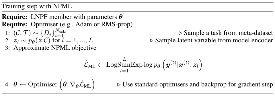
Fig. 32 Pseudo-code for a single training step of a LNPF member with NPML.
NPML is conceptually very simple as it directly approximates the training procedure of the CNPF, in the sense that it targets the same predictive likelihood during training. Moreover, it tends to work well in practice, typically leading to models achieving good performance. However, it suffers from two important drawbacks:
Bias: When applying the Monte-Carlo approximation, we have employed an unbiased estimator to the predictive likelihood. However, in practice we are interested in the log likelihood. Unfortunately, the log of an unbiased estimator is not itself unbiased. As a result, NPML is a biased (conservative) estimator of the true log-likelihood.
High Variance: In practice it turns out that NPML is quite sensitive to the number of samples \(L\) used to approximate it. In both our GP and image experiments, we find that on the order of 20 samples are required to achieve “good” performance. Of course, the computational and memory costs of training scale linearly with \(L\), often limiting the number of samples that can be used in practice.
Unfortunately, decreasing the number of samples \(L\) needed to perform well turns out to be quite difficult, and is an open question in training latent variable models in general. However, we next describe an alternative training procedure that typically works well with fewer samples.
Neural Process Variational Inference (NPVI)
NPVI is a training procedure proposed by [GSR+18], which takes inspiration from the literature on variational inference (VI). The central idea behind this objective function is to use posterior sampling to reduce the variance of NPML. For a better intuition regarding this, note that NPML is defined using an expectation against \(p_{\theta}(\mathbf{z} | \mathcal{C})\). The idea in posterior sampling is to use the whole task, including the target set, \(\mathcal{D} = \mathcal{C} \cup \mathcal{T}\) to produce the distribution over \(\mathbf{z}\), thus leading to more informative samples and lower variance objectives.
In our case, the posterior distribution from which we would like to sample is \(p(\mathbf{z} | \mathcal{C}, \mathcal{T})\), i.e., the distribution of the latent variable having observed both the context and target sets. Unfortunately, this posterior is intractable. To address this, [GSR+18] propose to replace the true posterior with simply passing both the context and target sets through the encoder, i.e.
Note\(\qquad p \left( \mathbf{z} | \mathcal{C}, \mathcal{T} \right) \neq p_{\theta} \left( \mathbf{z} | \mathcal{D} \right)\)
Note that these two distributions are different. We can compute \(p_{\theta} \left( \mathbf{z} | \mathcal{D} \right)\) by simply passing both \(\mathcal{C}\) and \(\mathcal{T}\) through the model encoder. One the other hand, the posterior \(p \left( \mathbf{z} | \mathcal{C}, \mathcal{T} \right)\) is computed using Bayes’ rule and our model definition:
Recalling that our decoder is defined by a complicated, non-linear neural network, we can see that this posterior is intractable, as it involves an integration against complicated likelihoods.
We can now derive the final objective function, which is a lower bound to the log marginal likelihood, by (i) introducing the approximate posterior as a sampling distribution, and (ii) employing a straightforward application of Jensen’s inequality.
where \(\mathrm{KL}(p \| q)\) is the Kullback-Liebler (KL) divergence between two distributions \(p\) and \(q\), and we have used the shorthand \(p_{\theta} \left( \mathbf{y}_{\mathcal{T}} | \mathbf{x}_{\mathcal{T}}, \mathbf{z} \right) = \prod_{t=1}^{T} p_{\theta} \left( y^{(t)} | x^{(t)}, \mathbf{z} \right)\) to ease notation. Let’s consider what we have achieved in Eq. (7).
Test Time
Of course, we can only sample from this approximate posterior during training, when we have access to both the context and target sets. At test time, we will only have access to the context set, and so the forward pass through the model will be equivalent to that of the model when trained with NPML, i.e., we will only pass the context set through the encoder. This is an important detail of NPVI: forward passes at meta-train time look different than they do at meta-test time!
Advanced\(\qquad\)LNPF as Amortised VI
The above procedure can be seen as a form of amortised VI. Amortised VI is a method for performing approximate inference and learning in probabilistic latent variable models, where an inference network is trained to approximate the true posterior distributions.
There are many resources available on (amortised) VI (e.g., Jaan Altosaar’s VAE tutorial, the Spectator’s take, or this review paper on modern VI), and we encourage readers unfamiliar with the concept to take the time to go through some of these. For our purposes, the following intuitions should suffice:
Assume that we have a latent variable model with a prior \(p(\mathbf{z})\), and a conditional likelihood for observations \(y\), written \(p_{\theta} \left(y | \mathbf{z} \right)\). The central idea in amortised VI is to introduce an inference network, denoted \(q_{\phi}(\mathbf{z} | y)\), which maps observations to distributions over \(\mathbf{z}\). We can then use \(q_{\phi}\) to derive a lower bound to the log-marginal likelihood, just as we did above:
In the VI terminology, this lower bound is commonly known as the evidence lower bound (ELBO). So maximising the ELBO with respect to \(\theta\) trains the model to optimise a lower bound on the log-marginal likelihood, which is a sensible thing to do. Moreover, it turns out that maximising the ELBO with respect to \(\phi\) minimises the KL divergence between \(q_{\phi} \left( \mathbf{z} | y \right)\) and the true posterior \(p_\theta(\mathbf{z} | y) = p_\theta(y | \mathbf{z}) p_\theta(\mathbf{z}) / p_\theta(y)\), so we can think of \(q_{\phi}\) as approximating the true posterior in a meaningful way.
In the NPF, to approximate the desired posterior, we can introduce a network that maps datasets to distributions over the latent variable. We already know how to define such networks in the NPF – that’s exactly what the encoder \(p_{\theta}(\mathbf{z} | \mathcal{C})\) does! In fact, NPVI proposes to use the encoder as the inference network when training LNPF members.
So we can view Eq.(7) as performing amortised VI for any member of the LNPF. The twist on standard amortised VI is that here, we are sharing \(q_{\phi}\) with a part of the model itself, since \(p_{\theta}(\mathbf{z} | \mathcal{D})\) plays the dual role of being an approximate posterior \(q_{\phi}\), and also defining the conditional prior having observed \(\mathcal{D}\). This somewhat complicates our understanding of the procedure, and could lead to unintended consequences.
When both the encoder and inference network parameterise Gaussian distributions over \(\mathbf{z}\) (as is standard), the KL-term can be computed analytically. Hence we can derive an unbiased estimator to Eq.(7) by taking samples from \(p_{\theta} \left( \mathbf{z} | \mathcal{D} \right)\) to estimate the first term on the RHS. Fig. 33 provides the pseudo-code for a single training iteration for a LNPF member, using NPVI as the target objective.
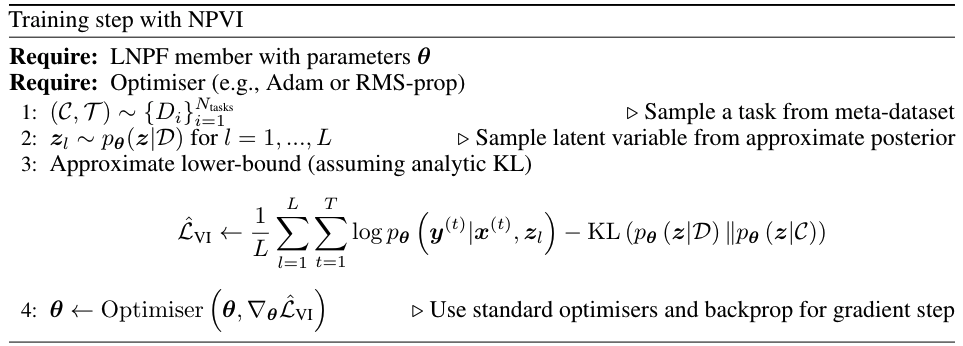
Fig. 33 Pseudo-code for a single training step of a LNPF member with NPVI.
Warning\(\qquad\)Biased estimators
Importantly, it is not the case that NPVI avoids the “biased estimator” issue of NPML. Rather, NPML defines a biased (conservative) estimator of the desired quantity, and NPVI produces an unbiased estimator of a strict lower-bound of the same quantity. In both cases, unfortunately, we do not have unbiased estimators of the quantity we really care about — \(\log p_{\boldsymbol\theta}(\mathbf{y}_\mathcal{T} | \mathbf{x}_\mathcal{T}, \mathcal{C})\).
Another consequence of this is that it is challenging to evaluate the models quantitatively, since our performance metrics are only ever lower bounds to the true model performance, and quantifying how tight those bounds are is quite challenging.
To better understand the NPVI objective, it is important to note — see the box below — that it can be rewritten as the difference between the desired log marginal likelihood and a KL divergence between approximate and true posterior:
The NPVI can thus be seen as maximizing the desired log marginal likelihood as well as forcing the approximate and true posterior to be similar.
Advanced\(\qquad\)Relationship between NPML and NPVI
There is a close relationship between the NPML and NPVI objectives. To see this, we denote the normalising constant for the distribution \(p_{\theta} \left( \mathbf{y}_{\mathcal{T}}, \mathbf{z} | \mathbf{x}_{\mathcal{T}}, \mathcal{C} \right)\) as
Now, we can rewrite the NPVI objective as
Thus, we can see that \(\mathcal{L}_{VI}\) is equal to \(\mathcal{L}_{ML}\) (with infinitely many samples) up to an additional KL term. This KL term has a nice interpretation as encouraging consistency among predictions with different context sets, which is the kind of consistency not baked into the NPF.
However, this term can also be a distractor. When dealing with NPF members, we are typically not interested in the latent variable \(\mathbf{z}\), and most considered tasks require only a “good” approximation to the predictive distribution over \(\mathbf{y}_{\mathcal{T}}\). Therefore, given only finite model capacity, and finite data, it may be preferable to focus all the model capacity on achieving the best possible predictive distribution (which is what \(\mathcal{L}_{ML}\) focuses on), rather than focusing on the distribution over \(\mathbf{z}\), as encouraged by the KL term introduced by \(\mathcal{L}_{VI}\).
Notice that if our approximate posterior can recover the true posterior, then the KL term is zero, and we are exactly optimising the log-marginal likelihood. In practice, however, the inequality holds, meaning that we are only optimising a lower-bound to the quantity we actually care about. Moreover, it is often quite difficult to know how tight this bound may be.
As we have discussed, the most appealing property of NPVI is that it utilises posterior sampling to reduce the variance of the Monte-Carlo estimator of the intractable expectation. This means that often we can get away with training models taking just a single sample, resulting in computationally and memory efficient training procedures. However, it also comes with several drawbacks, which can be roughly summarised as follows:
NPVI is focused on approximating the posterior distribution (see Eq.(8) ). However, in the NPF setting, we are typically only interested in the predictive distribution \(p(\mathbf{y}_T | \mathbf{x}_T, \mathcal{C})\), and it is unclear whether focusing our efforts on \(\mathbf{z}\) is beneficial to achieving higher quality predictive distributions.
In NPVI, the encoder plays a dual role: it is both part of the model, and used for posterior sampling. This fact introduces additional complexities in the training procedure, and it may be that using the encoder as an approximate posterior has a detrimental effect on the resulting predictive distributions.
As we shall see below, it is often the case that models trained with NPML produce better fits than equivalent models trained with NPVI, at the cost of additional computational and memory costs of training. Moreover, using NPVI often requires additional tricks and contraints to get good descent performance.
Armed with procedures for training LNPF-members, we turn our attention to the models themselves. In particular, we next introduce the latent-variable variant of each of the conditional models introduced in the previous section, and we shall see that having addressed the training procedures, the extension to latent variables is quite straightforward from a practical perspective.
Latent Neural Process (LNP)
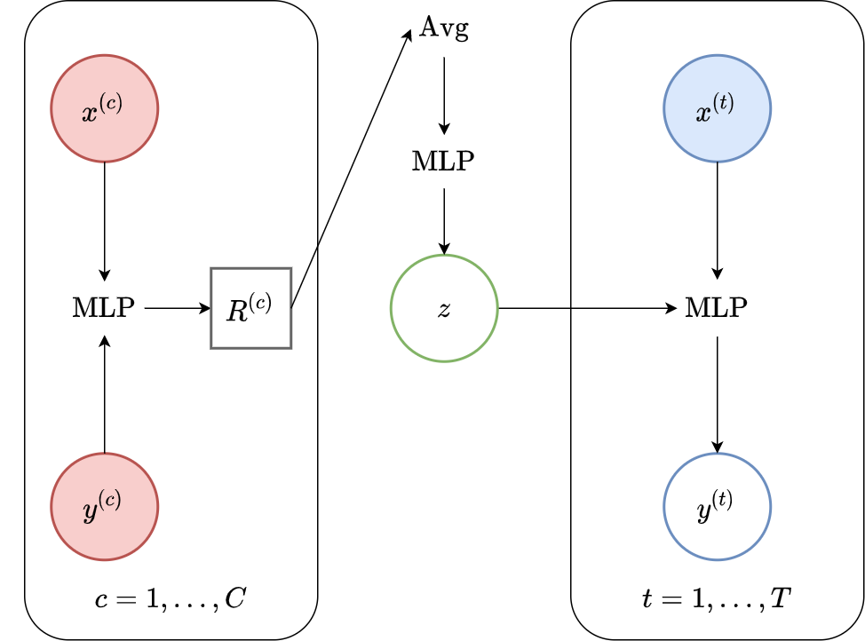
Fig. 34 Computational graph for LNPS.
The latent neural process [GSR+18] is the latent counterpart of the CNP, and the first member of the LNPF proposed in the literature. Given the vector \(R\), which is computed as in the CNP, we simply pass it through an additional MLP to predict the mean and variance of the latent representation \(\mathbf{z}\), from which we can produce samples. The decoder then has the same architecture as that of the CNP, and we can simply pass samples of \(\mathbf{z}\), together with desired target locations, to produce our predictive distributions. Fig. 34 illustrates the computational graph of the LNP.
Implementation\(\qquad\)Parameterising the Observation Noise
An important detail in the parameterisation of LNPF members is how the predictive standard deviation is handled, there are 2 possibilities
Heteroskedastic noise: As with CNPF members, the decoder parameterises a mean \(\mu^{(t)}\) and a standard deviation \(\sigma^{(t)}\) for each target location \(x^{(t)}\).
Homoskedastic noise: The decoder only parameterises a mean \(\mu^{(t)}\), while the standard deviation \(\sigma\) is a global (learned) observation noise parameter, i.e., it is shared for all target locations. Note that the uncertainty of the posterior predictive at two different target locations can still be very different. Indeed, it is influenced by the variance in the means \(\mu^{(t)}\), which arises from the uncertainty in the latent variable.
In practice, a heteroskedastic noise usually performs better than the homoskedastic variant.
Implementation\(\qquad\)”Lower Bounding” Standard Deviations
In the LNPF literature, it is common to “lower bound” the standard deviations of distributions output by models. This is often achieved by parameterising the standard deviation as
where \(\epsilon\) is a small real number (e.g. 0.001), and \(f_\sigma\) is the log standard deviation output by the model. This “lower bounding” is often used in practice for the standard deviations of both the latent and predictive distributions. In fact Le et al.[LKG+18] find that this consistently improves performance of the AttnLNP, and recommend it as best practice. Following the literature, the results displayed in this tutorial all employ such lower bounds. However, we note that, in our opinion, there is no conceptual justification for this trick, and it is indicative of flaws in the models and or training procedures.
Throughout the section we train LNPs with NPVI as in the original paper. Below, we show the predictive distribution of an LNP trained on samples from the RBF-kernel GP, as the number of observed context points from the underlying function increases.
Fig. 35 Samples from posterior predictive of LNPs (Blue) and the oracle GP (Green) with RBF kernel.
Fig. 31 shows that the latent variable indeed enables coherent sampling from the posterior predictive. In fact, within the range \([-1, 1]\) the model produces very nice samples, that seem to properly mimic those from the underlying process. Nevertheless, here too we see that the LNP suffers from the same underfitting issue as discussed with CNPs. We again see the tendency to overestimate the uncertainty, and often not pass through all the context points with the mean functions. Moreover, we can observe that beyond the \([-1, 1]\), the model seems to “give up” on the context points and uncertainty, despite having been trained on the range \([-2, 2]\).
Note\(\qquad\)NPVI vs NPML
In the main text we trained LNP with NPVI as in the original paper, we compare the results with NPML on different kernels below.
Fig. 36 Predictive distributions of LNPs (Blue) and the oracle GP (Green) with (top) RBF, (center) periodic, and (bottom) Noisy Matern kernels. Models were trained with (left) NPML and (right) NPVI.
Fig. 36 illustrates several interesting points that we tend to see in our experiments. First, as with the CNP, the model tends to underfit, and in particular fails catastrophically with the periodic kernel. In some cases, e.g., when trained on the RBF kernel with NPVI, the model seems to collapse the uncertainty arising from the latent variable in certain regions, and rely entirely on the observation noise. In our experiments, we observe that this tends to occur when training with NPVI, but not with NPML. Finally, we can see that NPML tends to produce predictive distributions that fit the data better, and tend to have lower uncertainty near the context set points.
Let us now consider the image experiments as we did with the CNP.
Fig. 37 samples (means conditioned on different samples from the latent) of the posterior predictive of a LNP on CelebA \(32\times32\) and MNIST. The last row shows the standard deviation of the posterior predictive corresponding to the last sample.
From Fig. 37 we see again that the latent variable enables relatively coherent sampling from the posterior predictive. As with the CNP, the LNP still underfits on images as is best illustrated when the context set is half the image.
Details
Model details, training and more plots in LNP Notebook. We also provide pretrained models to play around with.
Attentive Latent Neural Process (AttnLNP)
The Attentive LNPs [KMS+19] is the latent counterpart of AttnCNPs. Differently from the LNP, the AttnLNP added a “latent path” in addition to (rather than instead of) the deterministic path. The latent path is implemented with the same method as LNPs, i.e. a mean aggregation followed by a parametrization of a Gaussian. In other words, even though the deterministic representation \(R^{(t)}\) is target specific, the latent representation \(\mathbf{z}\) is target independent as seen in the computational graph (Fig. 38).
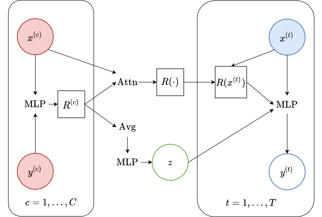
Fig. 38 Computational graph for AttnLNPS.
Throughout the section we train AttnLNPs with NPVI as in the original paper. Below, we show the predictive distribution of an AttnLNP trained on samples from RBF, periodic, and noisy Matern kernel GPs, again viewing the predictive as the number of observed context points is increased.
Fig. 39 Samples Posterior predictive of AttnLNPs (Blue) and the oracle GP (Green) with RBF,periodic, and noisy Matern kernel.
Fig. 39 paints an interesting picture regarding the AttnLNP. On the one hand, we see that it is able to do a significantly better job in modelling the marginals than the LNP. However, on closer inspection, we can see several issues with the resulting distributions:
Kinks: The samples do not seem to be smooth, and we see “kinks” that are similar (though even more pronounced) than in Fig. 14.
Collapse to AttnCNP: In many places the AttnLNP seems to collpase the distribution around the latent variable, and express all its uncertainty via the observation noise. This tends to occur more often for the AttnLNP when trained with NPVI rather than NPML.
Note\(\qquad\)NPVI vs NPML
As with the LNP, we compare the performance of the AttnLNP when trained with NPVI and NPML.
Fig. 40 Predictive distributions of AttnLNPs (Blue) and the oracle GP (Green) with (top) RBF, (center) periodic, and (bottom) Noisy Matern kernels. Models were trained with (left) NPML and (right) NPVI.
Here we see that the AttnLNP tends to “collapse” for both the RBF and noisy Matern kernels when trained with NPVI. In contrast, when trained with NPML it tends to avoid this behaviour. This is consistent with what we observe more generally in our experiments.
Let us now consider the image experiments as we did with the AttnCNP.
Fig. 41 Samples from posterior predictive of an AttnCNP for CelebA \(32\times32\), MNIST, ZSMM.
From Fig. 41 we see that AttnLNP generates quite impressive samples, and exhibits descent sampling and good performances when the model does not require generalisation (CelebA \(32\times32\), MNIST). However, as expected, the model “breaks” for ZSMM as it still cannot extrapolate.
Details
Model details, training and more plots in AttnLNP Notebook. We also provide pretrained models to play around with.
Convolutional Latent Neural Process (ConvLNP)
The Convolutional LNP [FBG+20] is the latent counterpart of the ConvCNP. In contrast with the AttnLNP, the latent path replaces the deterministic one (as with LNP), resulting in a latent functional representation (a latent stochastic process) instead of a latent vector valued variable.
Another way of viewing the ConvLNP, which is useful in gaining an intuitive understanding of the computational graph (see Fig. 42) is as consisting of two stacked ConvCNPs: the first takes in context sets and outputs a latent stochastic process. The second takes as input a sample from the latent process and models the posterior predictive conditioned on that sample.
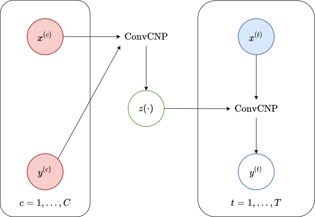
Fig. 42 Computational graph for ConvLNPs.
Implementation\(\qquad\)ConvLNP without ConvCNP
In our implementation we do not use two ConvCNPs to implement the ConvLNP. Instead, we use the same computational graph than for ConvCNPs but split the CNN into two. The output of the first CNN is a mean and a (log) standard deviation at every position of the (discrete) signal, which are then used to parametrize independent Gaussian disitrubtions each positions. The second CNN gets as input a sample from the first one, i.e., a discrete signal.
The computational graph for this implementation is shown in Fig. 43. Importantly both are mathematically equivalent, but using two ConvCNPs can be easier to understand and more modular, while using two CNNs avoids unecessary computations.
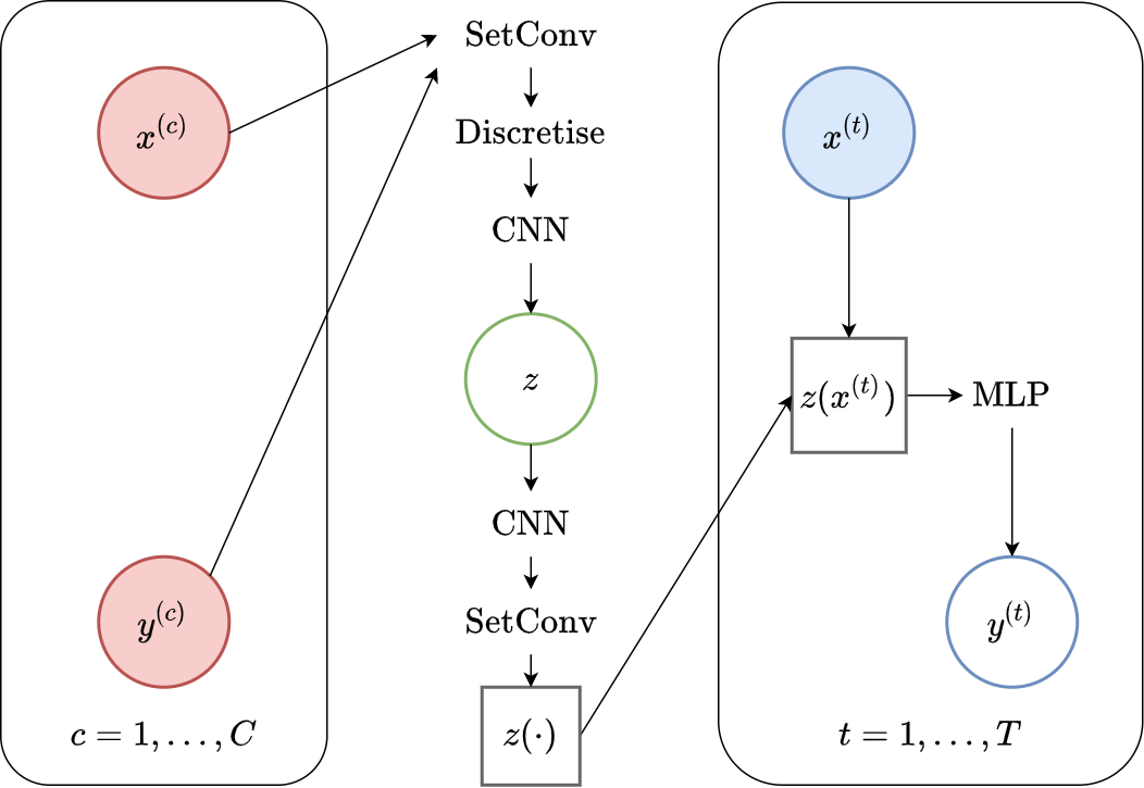
Fig. 43 Computational graph for ConvLNPs without using ConvCNPs.
One difficulty arises in training the ConvLNP with the NPVI objective, as it requires evaluating the KL divergence between two stochastic processes, which is a tricky proposition. [FBG+20] propose a simple approach, that approximates this quantity by instead summing the KL divergences at each discretisation location. However, as they note, the ConvLNP performs significantly better in most cases when trained with NPML rather than NPVI. Throughout this section we will thus use NPML instead of NPVI.
Note\(\qquad\)Global Latent Representations
In this tutorial, we consider a simple extension to the ConvLNP proposed by Foong et. al [FBG+20], which includes a global latent representation as well. The global representation is computed by average-pooling half of the channels in the latent function, resulting in a translation invariant latent representation, in addition to the translation equivariant one. The intuition behind such a representation is that it may help to capture aspects of the underlying function that are global, allowing the functional representation to represent more localised information. This intuition is clearest when considering the mixture of GPs experiments discussed below.
Fig. 44 Samples Posterior predictive of ConvLNPs (Blue) and the oracle GP (Green) with RBF,periodic, and noisy Matern kernel.
From Fig. 44 we see that ConvLNP performs very well and the samples are reminiscent of those from a GP, i.e., with much richer variability compared to Fig. 39. Further, as in the case of the ConvCNP, we see that the ConvLNP elegantly generalises beyond the range in \(X\)-space on which it was trained.
Note\(\qquad\)NPVI vs NPML
As with the LNP, we compare the performance of the ConvLNP when trained with NPVI and NPML. Note that to train ConvLNP with make NPVI it is important to decrease the dimensionality of the latent functional representation to decrease the KL term. Here we use 16 latent channels (for NPVI and NPML) instead of the usual 128.
Fig. 45 Predictive distributions of ConvLNP (Blue) and the oracle GP (Green) with (top) RBF, (center) periodic, and (bottom) Noisy Matern kernels. Models were trained with (left) NPML and (right) NPVI.
We see that a ConvLNP trained with NPML seems to gives better uncertainty estimates than when trained with NPVI.
Next, we consider the more challenging problem of having the ConvLNP model a stochastic process whose posterior predictive is non Gaussian. We do so by having the following underlying generative process: first, sample one of the 3 kernels discussed above, and second, sample a function from the sampled kernel. Importantly, the data generating process is a mixture of GPs, and the true posterior predictive process (achieved by marginalising over the different kernels) is non-Gaussian.
Fig. 46 demonstrates that ConvLNP performs quite well in this harder setting. Indeed, it seems to model the predictive process using the periodic kernel when the number of context points is small but quickly (around 10 context points) recovers the correct underlying kernel. Note how in the middle plot, the ConvLNP becomes progressively more and more “confident” that the process is periodic as more data is observed. Note that in Fig. 46 we are plotting the posterior predictive for the sampled GP, rather than the actual, non-GP posterior predictive process.
Again, we consider the performance of the ConvLNP in the image setting. In Fig. 47 we see that the ConvLNP does a reasonable job producing samples when the context sets are uniformly subsampled from images, but struggles with the “structured” context sets, e.g. when the left or bottom halves of the image are missing. Moreover, the ConvLNP is able to produce samples in the generalisation setting (ZSMM), but these are not always coherent, and include some strange artifacts that seem more similar to sampling the MNIST “texture” than coherent digits.
Fig. 47 Samples from posterior predictive of an ConvCNP for CelebA \(32\times32\), MNIST, ZSMM.
As discussed in the ‘Issues with the CNPF’ section, members of the CNPF could not be used to generate coherent samples, nor model non-Gaussian posterior predictive distributions. In contrast, Fig. 48 (right) demonstrates that, as expected, ConvLNP is able to produce non-Gaussian predictives for pixels, with interesting bi-modal and heavy-tailed behaviours.
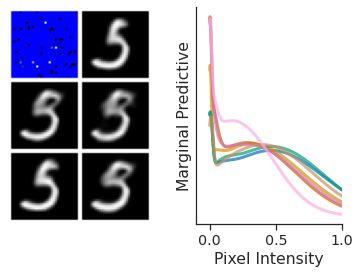
Fig. 48 Samples form the posterior predictive of ConvCNPs on MNIST (left) and posterior predictive of some pixels (right).
From Fig. 41 we see that AttnLNP generates quite impressive samples, and exhibits descent sampling and good performances when the model does not require generalisation (CelebA \(32\times32\), MNIST). However, as expected, the model “breaks” for ZSMM as it still cannot extrapolate.
Details
Model details, training and more plots in AttnLNP Notebook. We also provide pretrained models to play around with.
Issues and Discussion
We have seen how members of the LNPF utilise a latent variable to define a predictive distribution, thus achieving structured and expressive predictive distributions over target sets. Despite these advantages, the LNPF suffers from important drawbacks:
The training procedure only optimises a biased objective or a lower bound to the true objective.
Approximating the objective function requires sampling, which can lead to high variance during training.
They are more memory and computationally demanding, requiring many samples to estimate the objective for NPML.
It is difficult to quantitatively evaluate and compare different models, since only lower bounds to the log predictive likelihood can be estimated.
Despite these challenges, the LNPF defines a useful and powerful class of models. Whether to deploy a member of the CNPF or LNPF depends on the task at hand. For example, if samples are not required for a particular application, and we have reason to believe a parametric distribution may be a good description of the likelihood, it may well be that a CNPF would be preferable. Conversely, it is crucial to use the LNPF if sampling or dependencies in the predictive are required, for example in Thompson sampling.