Conditional NPF
Overview
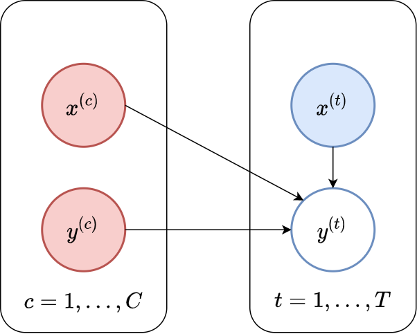
Fig. 6 Probabilistic graphical model for the Conditional NPF.
The key design choice for NPs is how to model the predictive distribution \(p_{\theta}( \mathbf{y}_\mathcal{T} | \mathbf{x}_\mathcal{T}; \mathcal{C})\). In particular, we require the predictive distributions to be consistent with each other for different \(\mathbf{x}_\mathcal{T}\), as discussed on the previous page. A simple way to ensure this is to use a predictive distribution that is factorised conditioned on the context set (as illustrated in Fig. 6). In other words, conditioned on the context set \(\mathcal{C}\), the prediction at each target location is independent of predictions at other target locations. We can concisely express this assumption as:
Advanced\(\qquad\)Factorisation \(\implies\) Consistency
We show that the CNPF predictive distribution specifies a consistent stochastic processes, given a fixed context set \(\mathcal{C}\). Recall that we require consistency under marginalisation and permutation.
(Consistency under permutation) Let \(\mathbf{x}_{\mathcal{T}} = \{ x^{(t)} \}_{t=1}^T\) be the target inputs and \(\pi\) be any permutation of \(\{1, ..., T\}\). Then the predictive density is:
since multiplication is commutative.
(Consistency under marginalisation) Consider two target inputs, \(x^{(1)}, x^{(2)}\). Then by marginalising out the second target output, we get:
which shows that the predictive distribution obtained by querying the CNPF member at \(x^{(1)}\) is the same as that obtained by querying it at \(x^{(1)}, x^{(2)}\) and then marginalising out the second target point. Of course, the same idea works with collections of any size, and marginalising any subset of the variables.
We refer to the sub-family of the NPF containing members that employ this factorisation assumption as the conditional Neural Process (sub-)Family (CNPF). A typical (though not necessary) choice is to set each \(p_{\theta} \left( y^{(t)} | x^{(t)}; \mathcal{C} \right)\) to be a Gaussian density. Now, recall that one guiding principle of the NPF is to encode the context set \(\mathcal{C}\) into a global representation \(R\), and then use a decoder to parametrise each \(p_{\theta} \left( y^{(t)} | x^{(t)}; \mathcal{C} \right)\). Putting these together, we can express the predictive distribution of CNPF members as
Where:
CNPF members make an important tradeoff. On one hand, the factorisation assumption places a severe restriction on the class of predictive stochastic processes we can model. As discussed at the end of this chapter, this has important consequences, such as the inability of the CNPF to produce coherent samples. On the other hand, the factorisation assumption makes evaluation of the predictive likelihoods analytically tractable. This means we can employ a simple maximum-likelihood procedure to train the model parameters, i.e., training amounts to directly maximising the log-likelihood \(\log p_{\theta}(\mathbf{y}_\mathcal{T} | \mathbf{x}_\mathcal{T}; \mathcal{C})\), as discussed on the previous page.
Now that we’ve given an overview of the entire CNPF, we’ll discuss three particular members: the Conditional Neural Process (CNP), Attentive Conditional Neural Process (AttnCNP), and the Convolutional Conditional Neural Process (ConvCNP). Each member of the CNPF can be broadly distinguished by:
The encoder \(\mathrm{Enc}_{\theta}: \mathcal{C} \mapsto R\), which has to be permutation invariant to treat \(\mathcal{C}\) as a set.
The decoder \(\mathrm{Dec}_{\theta}: R,x^{(t)} \mapsto \mu^{(t)},\sigma^{2(t)}\), which parametrizes the predictive distribution at location \(x^{(t)}\) using the global representation \(R\).
We begin by describing the Conditional Neural Process, arguably the simplest member of the CNPF, and the first considered in the literature.
Conditional Neural Process (CNP)
The main idea of the Conditional Neural Process (CNP) [GRM+18] is to enforce permutation invariance of the encoder by first locally encoding each context input-output pair into \(R^{(c)}\), and then aggregating the local encodings into a global representation, \(R\), of the context set using a commutative operation. Specifically, the local encoder is a feedforward multi-layer perceptron (MLP), while the aggregator is a mean pooling. The decoder is simply an MLP that takes as input the concatenation of the representation and the target input, \([R; x^{(t)}]\), and outputs a predictive mean \(\mu^{(t)}\) and variance \(\sigma^{2(t)}\).
Implementation\(\qquad\)Log Std
Typically, we parameterise \(\mathrm{Dec}_{\theta}\) as outputting \((\mu^{(t)}, \log \sigma^{(t)})\), i.e., the log standard deviation, so as to ensure that no negative variances occur.
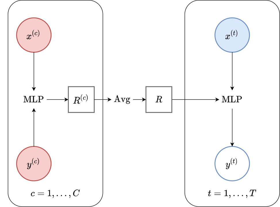
Fig. 7 Computational graph for CNPs.
To summarise, the CNP is defined by the following design choices (see Fig. 7):
Encoding: \(R = \mathrm{Enc}_{\theta}(\mathcal{C}) = \frac{1}{C} \sum_{c=1}^{C} \mathrm{MLP} \left( [x^{(c)}; y^{(c)}] \right)\) .
Decoding: \((\mu^{(t)}, \sigma^{2(t)}) = \mathrm{Dec}_{\theta}(R,x^{(t)}) = \mathrm{MLP} \left( [R,x^{(t)}] \right)\).
Note that the encoder is permutation invariant due to the commutativity of the sum operation, i.e., the order does not matter. Importantly, if the local encoder and the decoder were universal function approximators (think of “infinitely wide” MLP and unconstrained dimension of \(R\)) the CNP would essentially be able to predict any mean \(\mu^{(t)}\) and variance \(\sigma^{2(t)}\) thanks to the local encoder+aggregator (DeepSets; [ZKR+17]).
Advanced\(\qquad\)Universality and DeepSets
There is a strong relationship between this local encoder+aggregator and a class of models known as DeepSets networks introduced by Zaheer et al.[ZKR+17]. In particular, Zaheer et al. show that (subject to certain conditions) any continuous function operating on sets (\(S\)) can be expressed as:
for appropriate functions \(\rho\) and \(\phi\). This is known as a “sum decomposition” or “Deep Sets encoding”. This result tells us that, as long as \(\rho\) and \(\phi\) are universal function approximators, this sum-decomposition can be done without loss of generality in terms of the class of permutation-invariant maps that can be expressed.
CNPs make heavy use this type of architecture. To highlight the similarities, we can express each of the mean and standard deviation functions of the CNP as
where \([\cdot ; \cdot ]\) is the concatenation operation. In fact, the only difference between the CNP form and the DeepSets of Zaheer et al. is the concatenation operation in \(\rho\), and the use of the mean for aggregation, rather than summation. It is possible to leverage this relationship to show that CNPs can recover any continuous mean and variance functions, which provides justification for the proposed architecture.
Fig. 8 shows a schematic animation of the forward pass of a CNP. We see that every \((x, y)\) pair in the context set (here with three datapoints) is locally encoded by an MLP \(e\). The local encodings \(\{r_1, r_2, r_3\}\) are then aggregated by a mean pooling \(a\) to a global representation \(r\). Finally, the global representation \(r\) is fed along with the target input \(x_{T}\) into a decoder MLP \(d\) to yield the mean and variance of the predictive distribution of the target output \(y\).
Fig. 8 Schematic representation of the forward pass of members of the CNP taken from Marta Garnelo. \(e\) is the local encoder MLP, \(a\) is a mean-pooling aggregation, \(d\) is the decoder MLP.
Notice that the computational cost of making predictions for \(T\) target points conditioned on \(C\) context points with this design is \(\mathcal{O}(T+C)\). Indeed, each \((x,y)\) pair of the context set is encoded independently (\(\mathcal{O}(C)\)) and the representation \(R\) can then be re-used for predicting at each target location (\(\mathcal{O}(T)\)). This means that once trained, CNPs are much more efficient than GPs (which scale as \(\mathcal{O}(C^3+T*C^2)\)).
Let’s see what prediction using a CNP looks like in practice. We first consider a simple 1D regression task trained on samples from a GP with a radial basis function (RBF) kernel (data details in Datasets Notebook). Besides providing useful (and aesthetically pleasing) visualisations, the GPs admit closed form posterior predictive distributions, which allow us to compare to the “best possible” distributions for a given context set. In particular, if the CNP was “perfect”, it would exactly match the predictions of the oracle GP.
Fig. 9 Predictive distribution of a CNP (the blue line represents the predicted mean function and the shaded region shows a standard deviation on each side \([\mu-\sigma,\mu+\sigma]\)) and the oracle GP (green line represents the ground truth mean and the dashed line show a standard deviations on each side) with RBF kernel.
Fig. 9 provides the predictive distribution for a CNP trained on many samples from such a GP. The figure demonstrates that the CNP performs quite well in this setting. As more data is observed, the predictions become tighter, as we would hope. Moreover, we can see that the CNP predictions quite accurately track the ground truth predictive distribution.
That being said, we can see some signs of underfitting: for example, the predictive mean does not pass through all the context points, despite there being no noise in the data-generating distribution. The underfitting becomes clear when considering more complicated kernels, such as a periodic kernel (i.e. GPs generating random periodic functions as seen in Datasets Notebook). One thing we can notice about the ground truth GP predictions is that it leverages the periodic structure in its predictions.
Fig. 10 Posterior predictive of a CNP (Blue line for the mean with shaded area for \([\mu-\sigma,\mu+\sigma]\)) and the oracle GP (Green line for the mean with dotted lines for +/- standard deviation) with Periodic kernel.
In contrast, we see that the CNP completely fails to model the predictive distribution: the mean function is overly smooth and hardly passes through the context points. Moreover, it seems that no notion of periodicity has been learned in the predictions. Finally, the uncertainty seems constant, and is significantly overestimated everywhere. It seems that the CNP has failed to learn the more complex structure of the optimal predictive distribution for this kernel.
Let’s now test the CNP (same architecture) on a more interesting task, one where we do not have access to the ground truth predictive distribution: image completion. Note that NPs can be used to model images, as an image can be viewed as a function from pixel locations to pixel intensities or RGB channels— expand the dropdown below if this is not obvious.
Note\(\qquad\)Images as Functions
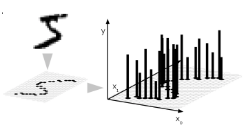
In the Neural-Process literature, and in this tutorial, we view images as real-valued functions on the two-dimensional plane. Each input \(x\) is a two-dimensional vector denoting pixel location in the image, and each \(y\) is a real number representing pixel intensity (or a three-dimensional vector for RGB images). Fig. 11 illustrates how to interpret an MNIST image as a function:
During meta-training, we treat each image as a sampled function, and split the image into context and target pixels. At test time, we can feed in a new context set and query the CNP at all the pixel locations, to interpolate the missing values / targets in the image. Fig. 12 shows the results:
Fig. 12 Posterior predictive of a CNP on CelebA \(32\times32\) and MNIST.
These results are quite impressive, however there are still some signs of underfitting. In particular, the interpolations are not very sharp, and do not totally resemble the ground truth image even when there are many context points. Nevertheless, this experiment demonstrates the power of neural processes: they can be applied out-of-the-box to learn this complicated structure directly from data, something that would be very difficult with a GP.
One potential solution to the overfitting problem, motivated by the universality of CNPs, is to increase the capacity of the networks \(\mathrm{Enc}_{\theta}\) and \(\mathrm{Dec}_{\theta}\), as well as increase the dimensionality of \(R\). Unfortunately, it turns out that the CNP’s modelling power scales quite poorly with the capacity of its networks. A more promising avenue, which we explore next, is to consider the inductive biases of its architectures.
Note
Model details and more plots, along with code for constructing and training CNPs, can be found in CNP Notebook. We also provide pretrained models to play around with.
Attentive Conditional Neural Process (AttnCNP)
One possible explanation for CNP’s underfitting is that all points in the target set share a single global representation \(R\) of the context set, i.e., \(R\) is independent of the location of the target input. This implies that all points in the context set are given the same “importance”, regardless of the location at which a prediction is being made. For example, CNPs struggle to take advantage of the fact that if a target point is very close to a context point, they will often both have similar values. One possible solution is to use a target-specific representation \(R^{(t)}\).
To achieve this, Kim et al. [KMS+19] propose the Attentive CNP (AttnCNP1), which replace CNPs’ mean aggregation by an attention mechanism [BCB15]. There are many great resources available about the use of attention mechanisms in machine learning (e.g. Distill’s interactive visualisation, Lil’Log, or the Illustrated Transformer), and we encourage readers unfamiliar with the concept to look through these. For our purposes, it suffices to think of attention mechanisms as learning to attend to specific parts of an input that are particularly relevant to the desired output, giving them more weight than others when making a prediction. Specifically, the attention mechanism is a function \(w_{\theta}(\cdot, \cdot)\) that weights each context point (the keys) for every target location (the querries), \(w_{\theta}(x^{(c)},x^{(t)})\). The AttnCNP then replaces CNPs’ simple average by a (more general) weighted average which gives a larger weight to “important” context points.
To illustrate how attention can alleviate underfitting, imagine that our context set contains two observations with inputs \(x^{(1)}, x^{(2)}\) that are “very far” apart in input space. These observations (input-output pairs) are then mapped by the encoder to the local representations \(R^{(1)}, R^{(2)}\) respectively. Intuitively, when making predictions close to \(x^{(1)}\), we should focus on \(R^{(1)}\) and ignore \(R^{(2)}\), since \(R^{(1)}\) contains much more information about this region of input space. An attention mechanism allows us to parameterise and generalise this intuition, and learn it directly from the data!
This gain in expressivity comes at the cost of increased computational complexity, from \(\mathcal{O}(T+C)\) to \(\mathcal{O}(T*C)\), as a representation of the context set now needs to be computed for each target point.
Functional Representation
Notice that the encoder \(\mathrm{Enc}_{\theta}\) does not take the target location \(x^{(t)}\) and can thus not directly predict a target-specific representation \(R^{(t)}\). To make the AttnCNP fit in an encoder – global representation – decoder framework we have to treat the global representation as a function of the form \(R : \mathcal{X} \to \mathbb{R}^{dimR}\) instead of a vector. In the decoder, this function will be queried at the target position \(x^{(t)}\) to yield a target specific vector representation \(R^{(t)} = R(x^{(t)})\).
To summarise, the AttnCNP is defined by the following design choices (see Fig. 13):
Encoding: \(R(\cdot) = \mathrm{Enc}_{\theta}(\mathcal{C}) = \sum_{c=1}^{C} w_{\theta} \left( x^{(c)}, \cdot \right) \mathrm{MLP} \left( [x^{(c)}; y^{(c)}] \right)\) .
Decoding: \((\mu^{(t)}, \sigma^{2(t)}) = \mathrm{Dec}_{\theta}(R, x^{(t)}) = \mathrm{MLP} \left( [R(x^{(t)}),x^{(t)}] \right)\).
Note that, as for the CNP, the encoder is permutation invariant due to the commutativity of the sum operation.
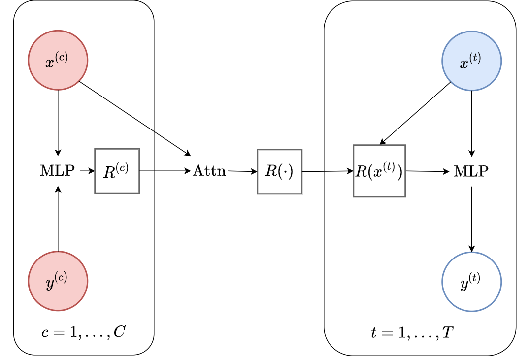
Fig. 13 Computational graph for AttnCNPs.
Note\(\qquad\)Self-Attention
In the above discussion we only consider an attention mechanism between the target and context set (referred to as cross-attention). In addition, AttnCNP often first uses an attention mechanism between context points: self-attention, i.e., the local encoding \(\mathrm{MLP} \left( [x^{(c)}; y^{(c)}] \right)\) is replaced by \(\sum_{c'=1}^{C} w_{\theta} \left( x^{(c')}, x^{(c)} \right) \mathrm{MLP} \left( [x^{(c')}; y^{(c')}] \right)\).
Notice that this does not impact the permutation invariance of the predictions — if the context set is permuted, so will the set of local representations. When cross-attention is applied, the ordering of this set is irrelevant, hence the predictions are unaffected.
Using a self-attention layer will also increase the computational complexity to \(\mathcal{O}(C(C+T))\) as each context point will first attend to every other context point in \(\mathcal{O}(C^2)\) before the cross attention layer which is \(\mathcal{O}(C*T)\).
Without further ado, let’s see how the AttnCNP performs in practice. We will first evaluate it on GP regression with different kernels (RBF, Periodic, and Noisy Matern).
Fig. 14 Posterior predictive of AttnCNPs (Blue line for the mean with shaded area for \([\mu-\sigma,\mu+\sigma]\)) and the oracle GP (Green line for the mean with dotted lines for +/- standard deviation) with RBF, Periodic, and Noisy Matern kernel.
Fig. 14 demonstrates that, as desired, AttnCNP alleviates many of the underfitting issues of the CNP, and generally performs much better on the challenging kernels. However, looking closely at the resulting fits, we can still see some dissatisfying properties:
The fit on the Periodic kernel is still not great. In particular, we see that the mean and variance functions of the AttnCNP often fail to track the oracle GP, as they only partially leverage the periodic structure.
The posterior predictive of the AttnCNP has “kinks”, i.e., it is not very smooth. Notice that these kinks usually appear between 2 context points. This leads us to believe that they are a consequence of the AttnCNP abruptly changing its attention from one context point to the other.
Overall, AttnCNP performs quite well in this setting. Next, we turn our attention (pun intended) to the image setting:
Fig. 15 Posterior predictive of an AttnCNP for CelebA \(32\times32\) and MNIST.
Fig. 15 illustrates the performance of the AttnCNP on image reconstruction tasks with CelebA (left) and MNIST (right). Note that the reconstructions are sharper than those for the CNP. Interestingly, when only a vertical or horizontal slice is shown, the ANP seems to “blur” out its reconstruction somewhat.
Note
Model details, training and more plots in AttnCNP Notebook. We also provide pretrained models to play around with.
Generalisation and Extrapolation
So far, we have seen that well designed CNPF members can flexibly model a range of stochastic processes by being trained from functions sampled from the desired stochastic process. Next, we consider the question of generalisation and extrapolation with CNPF members.
Let’s begin by discussing these properties in GPs. Many GPs used in practice have a property known as stationarity. Roughly speaking, this means that the GP gives the same predictions regardless of the absolute position of the context set in input space — only relative position matters. One reason this is useful is that stationary GPs will make sensible predictions regardless of the range of the inputs you give it. For example, imagine performing time-series prediction. As time goes on, the input range of the data increases. Stationary GPs can handle this without any issues.
In contrast, one downside of the CNP and AttnCNP is that it learns predictions solely through the data that it is presented with during meta-training. If this data has a limited range in input space, then there is no reason to believe that the CNP or AttnCNP will be able to make sensible predictions when queried outside of this range. In fact, we know that neural networks are typically quite bad at generalising outside their training distribution, i.e., in the out-of-distribution (OOD) regime.
Let’s first probe this question on the 1D regression experiments. To do so, we examine what happens when the context and target set contains points located outside the training range.
Fig. 16 Extrapolation of posterior predictive of CNP (Top) and AttnCNP (Bottom) and the oracle GP (Green) with RBF kernel. Left of the red vertical line is the training range, everything to the right is the “extrapolation range”.
Fig. 16 clearly shows that the CNP and the AttnCNP break as soon as the target and context points are outside the training range. In other words, they are not able to model the fact that the RBF kernel is stationary, i.e., that the absolute position of target points is not important, but only their relative position to the context points. Interestingly, they both fail in different ways: the CNP seems to fail for any target location, while the AttnCNP fails only when the target locations are in the extrapolation regime — suggesting that it can deal with context set extrapolation.
We can also observe this phenomenon in the image setting. For example let us evaluate the CNP and AttnCNP on Zero Shot Multi MNIST (ZSMM) where the training set consists of translated MNIST examples, while the test images are larger canvases with 2 digits. Refer to Datasets Notebook for training and testing examples.
Again we see in Fig. 17 and Fig. 18 that the models completely break in this generalisation task. They are unable to spatially extrapolate to multiple, uncentered digits. This is likely not surprising to anyone who has worked with neural nets as the test set here is significantly different of the training set. Despite the challenging nature of this task, it turns out that we can in fact construct NPs that perform well, by building in the appropriate inductive biases. This leads us to our next CNPF member — the ConvCNP.
Convolutional Conditional Neural Process (ConvCNP)
Disclaimer
The authors of this tutorial are co-authors on the ConvCNP paper.
Translation Equivariance (TE)
It turns out that the type of generalisation we are looking for — that the predictions of NPs depend on the relative position in input space of context and target points rather than the absolute one — can be mathematically expressed as a property called translation equivariance (TE). Intuitively, TE states that if our observations are shifted in input space (which may be time, as in audio waveforms, or spatial coordinates, as in image data), then the resulting predictions should be shifted by the same amount. This simple inductive bias, when appropriate, is extremely effective. For example, convolutional neural networks (CNNs) were explicitly designed to satisfy this property [FM82][LBD+89], making them the state-of-the-art architecture for spatially-structured data.
In Fig. 19, we visualise translation equivariance in the setting of stochastic process prediction. Here, we show stationary GP regression, which leads to translation equivariant predictions. We can see that as the context set is translated, i.e., all the data points in \(\mathcal{C}\) are shifted in input space by the same amount, so is the resulting predictive distribution. To achieve spatial generalisation, we would like this property also to hold for neural processes.
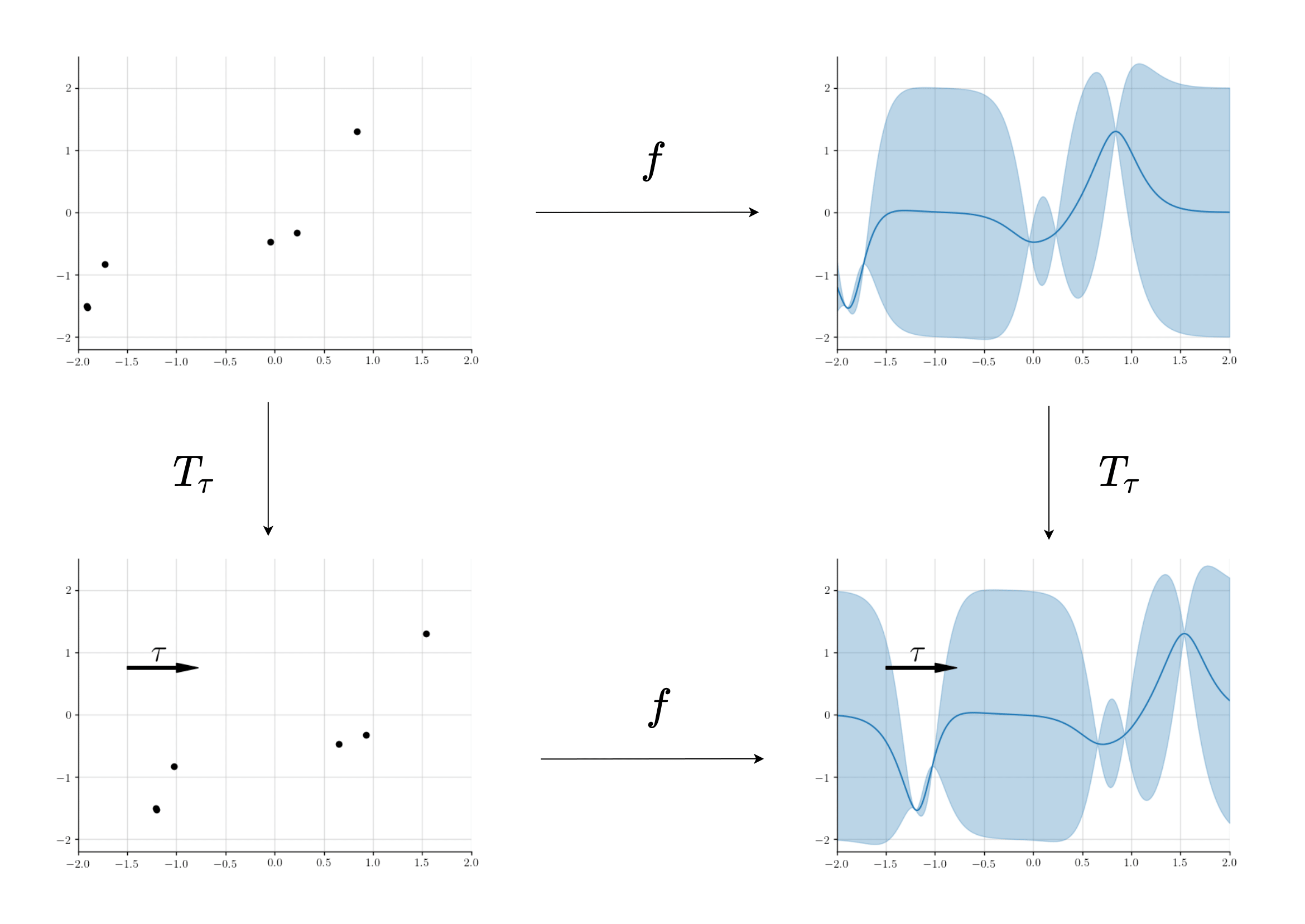
Fig. 19 Example of a translation equivariant mapping from a dataset to a predictive stochastic process.
Advanced\(\qquad\)Translation equivariance
More precisely, translation equivariance is a property of a map between two spaces, where each space has a notion of translation defined on it (more precisely, there is a group action of the translation group on each space). In the CNPF case, the input space \(\mathcal{Z}\) is the space of finite datasets, such that each \(Z \in \mathcal{Z}\) can be written as \(Z = \{(x_n, y_n)\}_{n=1}^N\) for some \(N \in \mathbb{N}\). The output space \(\mathcal{H}\) is a space of continuous functions on \(\mathcal{X}\), where \(\mathcal{X}\) is the input domain of the regression problem (e.g., time, spatial position). Think of \(\mathcal{H}\) as the set of all possible predictive mean and variance functions. The map acting from \(\mathcal{Z}\) to \(\mathcal{H}\) is then the CNPF member itself.
Let \(\tau \in \mathcal{X}\) be a translation vector. We define translations on each of these spaces as:
Then, a mapping \(f \colon \mathcal{Z} \to \mathcal{H}\) is said to be translation equivariant if \(f(T_\tau Z) = T'_\tau f(Z)\) for all \(\tau \in \mathcal{X}\) and \(Z \in \mathcal{Z}\). In other words, “shifting then predicting” gives the same result as “predicting then shifting”.
ConvCNP
This provides the central motivation behind the ConvCNP [GBF+20]: baking TE into the CNPF, whilst preserving its other desirable properties. Specifically, we would like the encoder to be a TE map between the context set \(\mathcal{C}\) and a functional representation \(R(\cdot)\), which as for AttnCNP will then be queried at the target location \(R^{(t)}=R(x^{(t)})\). In deep learning, the prime candidate for a TE encoder is a CNN. There is however an issue: the inputs and outputs to a CNN are discrete signals (e.g. images) and thus cannot take as input sets nor can they be queried at continuous (target) location \(x^{(t)}\). Gordon et al. [GBF+20] solve this issue by introducing the SetConv layer, an operation which extends standard convolutions to sets and could be very useful beyond the NPF framework.
SetConv
Standard convolutional layers in deep learning take in a discrete signal/function (e.g. a \(128\times128\) monochrome image that can be seen as a function from \(\{0, \dots , 127\}^2 \to [0,1]\)) and outputs a discrete signal/function (e.g. another \(128\times128\) monochrome image). The SetConv layer extends this operation to sets, i.e., it takes as input a set of continuous input-output pairs \(\{(x^{(c)},y^{(c)})\}_{c=1}^{C}\) (e.g. a time-series sampled at irregular points) and outputs a function that can be queried at continuous locations \(x\).
Here, \(w_{\theta}\) is a function that maps the distance between \(x^{(c)}\) and \(x\) to a real number. It is most often chosen to be an RBF: \(w_{\theta}(r) = \exp(- \frac{\|r\|^2_2}{\ell^2} )\), where \(\ell\) is a learnable lengthscale parameter. You can think of this operation as simply placing Gaussian bumps down at every datapoint, similar to Kernel Density Estimation.
Note that the SetConv operation is permutation invariant due to the sum operation.Furthermore, it is very similar to an attention mechanism, the main difference being that:
The weight only depends on the distance \(x^{(c)}-x\) rather than on their absolute values. This is the key for TE, which intuitively requires the mapping to only depend on relative positions rather than absolute ones.
We append a constant 1 to the value, \(\begin{bmatrix} 1 \\ y^{(c)} \end{bmatrix}\), which results in an additional channel. Intuitively, we can think of this additional channel — referred to as the density channel — as keeping track of where data was observed in \(\mathcal{C}\).
Note\(\qquad\)Density Channel
To better understand the role of the density channel, consider a context set containing a point \((x^{(c')}, y^{(c')})\), with \(y^{(c')} = 0\). Without the density channel, this point would have no impact on the output of the SetConv:
Hence, without a density channel, the encoder would be unable to distinguish between observing a context point with \(y^{(c)} = 0\), and not observing a context point at all! With the density channel, the contribution of the point \(c'\) becomes non-zero, specifically it contributes \(\begin{bmatrix} w_{\theta} \left( x - x^{(c)} \right) \\ 0 \end{bmatrix}\) to the predictions. This turns out to be important in practice, as well as in the theoretical proofs regarding the expressivity of the ConvCNP.
Note\(\qquad\)Normalisation
It is common practice to use the density channel to normalise the output of the non-density channels (also called the signal channels), so that the functional encoding becomes:
Intuitively, this ensures that the magnitude of the signal channel doesn’t blow up if there are a large number of context points at the same spot. The density channel of the ConvCNP encoder can be seen as (a scaled version of) a kernel density estimate, and the normalised signal channel can be seen as Nadaraya-Watson kernel regression.
Note that if \(x^{(c)},x^{(t)}\) are discrete, the SetConv essentially recovers the standard convolutional layer, denoted Conv. For example, let \(I\) be a \(128\times128\) monochrome image, then
for all pixel locations \(x^{(t)} \in \{0, \dots , 127\}^2 \), where \(1\) comes from the fact that the density channel is always \(1\) when their are no “missing values”.
Armed with this convolution mapping a set to continuous a function, we can use a CNN as our encoder by “wrapping it” around two SetConvs. Specifically, the encoder of the ConvCNP first uses a SetConv to ensure that the encoder can take the context set \(\mathcal{C}\) as input. The output of the SetConv (a continuous function) is then discretised — by evaluating it at an evenly spaced grid of input locations \(\{ \mathrm{SetConv}\left( \mathcal{C} \right)(x^{(u)}) \}_{u=1}^U\) — so that it can be given as input to a CNN. Finally the output of the CNN (a discrete function) is passed through an additional SetConv to obtain a continuous functional representation \(R\).
Warning
The discretisation means that the resulting ConvCNP can only be approximately TE, where the quality of the approximation is controlled by the number of points \(U\). If the spacing between the grid points is \(\Delta\), the ConvCNP would not be expected to be equivariant to shifts of the input that are smaller than \(\Delta\).
Similarly to AttnCNP, the decoder applies the resulting functional representation to the target location to get a target specific representation \(R^{(t)}=R(x^{(t)})\), which is then used by an MLP to parametrize the final Gaussian distribution. The only difference with AttnCNP being that the MLP does not directly take \(x^{(t)}\) as input, to ensure that the ConvCNP is TE.
Putting everything together, we can define the ConvCNP using the following design choices (illustrated in Fig. 20):
Encoding: \(R(\cdot) = \mathrm{Enc}_{\theta}(\mathcal{C}) = \mathrm{SetConv} \left( \mathrm{CNN}\left(\{ \mathrm{SetConv}\left( \mathcal{C} \right)(x^{(u)}) \}_{u=1}^U \right) \right)\) .
Decoding: \((\mu^{(t)}, \sigma^{2(t)}) = \mathrm{Dec}_{\theta}(R, x^{(t)}) = \mathrm{MLP} \left( R(x^{(t)}) \right)\).
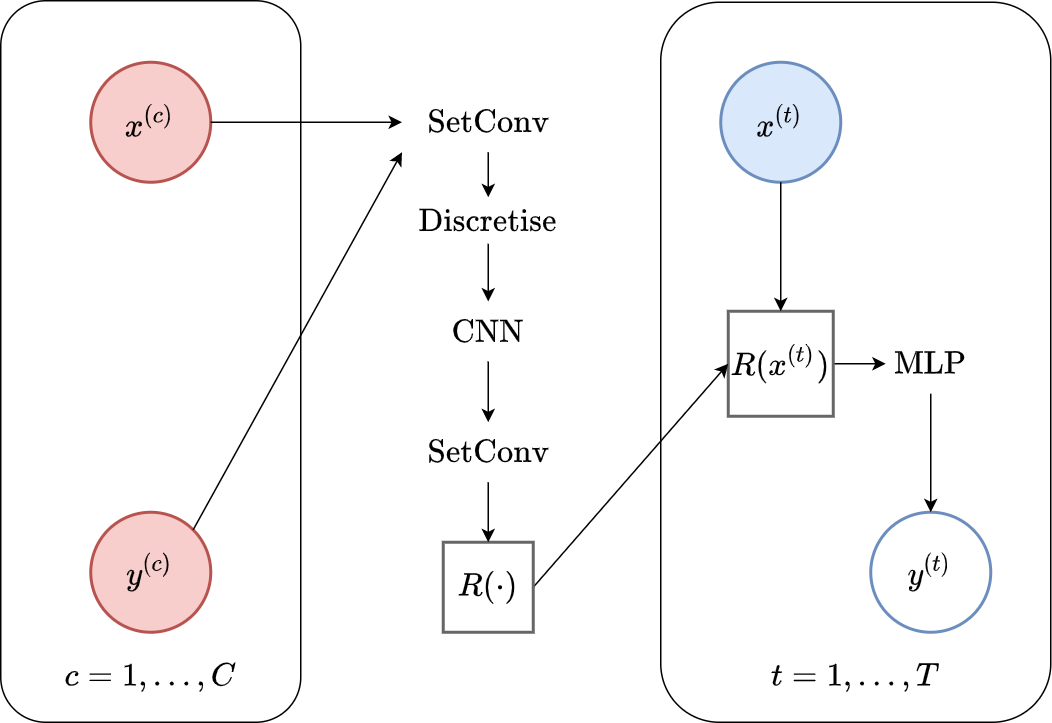
Fig. 20 Computational graph of ConvCNP.
Disclaimer\(\qquad\) Encoder vs Decoder
Note that the separation of the ConvCNP into encoder and decoder is somewhat arbitrary. You could also view the encoder as the first SetConv, and the decoder as the CNN with the second SetConv, which is the view presented in the original ConvCNP paper.
Importantly, if the CNN was a universal function approximator (think about “infinite channels” in the CNN and \(U \to \infty\)) the ConvCNP would essentially be able to predict any mean \(\mu^{(t)}\) and variance \(\sigma^{2(t)}\) that can be predicted with a TE map (ConvDeepSets; [GBF+20]).
Advanced\(\qquad\)ConvDeepSets
Similar to how CNPs make heavy use of “DeepSet” networks, ConvCNPs rely on the ConvDeepSet architecture which was also proposed by Gordon et al. [GBF+20]. ConvDeepSets map sets of the form \(Z = \{(x_n, y_n)\}_{n=1}^N\), \(N \in \mathbb{N}\) to a space of functions \(\mathcal{H}\), and have the following form
for appropriate functions \(\phi\), and \(w_{\theta}\), and \(\rho\) translation equivariant. The key result of Gordon et al. is to demonstrate that not only are functions of this form translation equivariant, but under mild conditions, any continuous and translation equivariant function on sets \(Z\) has a representation of this form. This result is analagous to that of Zaheer et al., but extended to translation equivariant functions on sets.
ConvCNPs then define the parameterisations of the mean and variance functions using ConvDeepSets. In particular, ConvCNPs specify \(\phi \colon y \mapsto (1, y)^T\), \(\rho\) as a CNN, and \(w_{\theta}\) as an RBF kernel, and use ConvDeepSets to parameterise the predictive mean and standard deviation functions. Thus, ConvDeepSets motivate the architectural choices of the ConvCNP analagously to how DeepSets can be used to provide justification for the CNP architecture.
Fig. 21 shows a schematic animation of the forward pass of a ConvCNP. We see that every \((x, y)\) pair in the context set (here with ten datapoints) goes through a SetConv. After concatenting the density channel, we discretize both the signal and the density channel so that they can be used as input to a CNN. The result then goes through a second SetConv to ouput a functional representation \(R(\cdot)\) which an be querried at any target location \(x^{(t)}\). Finally, the global representation evaluated at each target \(R(x^{(t)})\) is fed into a decoder MLP to yield the mean and variance of the predictive distribution of the target output \(y\).
Fig. 21 Schematic representation of the forward pass of members of the ConvCNP.
Implementation\(\qquad\)On-the-grid ConvCNP
The architecture described so far is referred to as the “off-the-grid” ConvCNP in the original paper, since it can handle input observations at any point on the \(x\)-axis. However, we sometimes have situations where inputs end up regularly spaced on the \(x\)-axis. A prime example of this is in image data, where the input image lives on a regularly-spaced 2D grid. For this case, the authors propose the “on-the-grid” ConvCNP, which is a simplified version that is easier to implement.
In the on-the-grid ConvCNP, the input data already lives on a discretised grid. Hence, after appending a density channel, this can immediately be fed into a CNN, without the need for SetConv’s. Suppose we have an image, represented as an \(H \times W\) matrix. Within this image, we have \(C\) observed pixels and \(HW - C\) unobserved pixels. We represent an observed pixel with the vector \([1, y^{(c)}]^T\), and an unobserved pixel with the vector \([0, 0]^T\). As before, the first element of this vector is the density channel, and indicates that a datapoint has been observed.
To implement this, let the input image be \(I \in \mathbb{R}^{H \times W}\). Let \(M \in \mathbb{R}^{H \times W}\) be a mask matrix, with \(M_{i,j} = 1\) if the pixel at location \((i,j)\) is in the context set, and \(0\) otherwise. Then we can compute the density channel as \(\mathrm{density} = M\) and the signal channel as \(\mathrm{signal} = I \odot M\), where \(\odot\) denotes element-wise multiplication. We then stack these matrices as \([\mathrm{density}, \mathrm{signal}]^T\). This can then be passed into a CNN, and the CNN can output one channel for the predictive mean, and another for the log predictive variance.
Note\(\qquad\)Computational Complexity
Computing the discrete functional representation requires considering \(C\) points in the context set for each discretised function location which scales as \(\mathcal{O}(U*C)\). Similarly, computing the predictive at the target inputs scales as \(\mathcal{O}(U*T)\). Finally, if the convolutional kernel has width \(K\), the complexity of the CNN scales as \(\mathcal{O}(U*K)\) — here we are ignoring the depth and number of channels. Hence the computational complexity of inference in a ConvCNP is \(\mathcal{O}(U(C+K+T))\). In the on-the-grid ConvCNP, the computational complexity is simply \(\mathcal{O}(U*K)\), where \(U\) is the number of pixels for image data.
This shows that there is a trade-off: if the number of discretisation points \(U\) is too large then the computational cost will not be manageable, but if it is too small then ConvCNP will be only very “coarsely” TE.
Now that we have constructed a translation equivariant member of the CNPF, we can test it in the more challenging extrapolation regime. We begin with the same set of GP experiments, but this time already including data observed from outside the original training range.
Fig. 22 Extrapolation (red dashes) of posterior predictive of ConvCNPs (Blue) and the oracle GP (Green) with (top) RBF, (center) periodic, and (bottom) Noisy Matern kernel.
Fig. 22 demonstrates that the ConvCNP indeed performs very well! In particular, we can see that:
Like the use of attention, the TE inductive bias also helps the model avoid the tendency to underfit the data.
Unlike the other members of the CNPF, the ConvCNP is able to extrapolate outside of the training range. Note that this is a direct consequence of TE.
Unlike attention, the ConvCNP produces smooth mean and variance functions, avoiding the “kinks” introduced by the AttnCNP.
The ConvCNP is able to learn about the underlying structure in the periodic kernel. We can see this by noting that it produces periodic predictions, even “far” away from the observed data.
Note\(\qquad\)Finite Receptive Field
The periodic kernel example is a little misleading, as the ConvCNP does not recover the underlying GP predictions everywhere. In fact, we know that it cannot exactly recover the underlying process. Indeed, it can only model local periodicity because it has a bounded receptive field — the size of the input region that can affect a particular output. See this Distill article for a further explanation of CNN receptive fields. This is best seen when considering a much larger target interval (\([-2,14]\) instead of \([0,4]\)):
Fig. 23 Large extrapolation (red dashes) of posterior predictive of ConvCNPs (Blue) and the oracle GP (Green) with periodic kernel.
In fact, this is true for any of the GPs above, all of which have “infinite receptive fields” — in principle, an observation at one point affects the predictions along the entire \(x\)-axis. This means that no model with a bounded receptive field can exactly recover the GP predictive distribution everywhere. In practice however, most GPs with non-periodic kernels (e.g., with RBF and Matern kernels) have a finite length-scale, and points much further apart than the length-scale are, for all practical purposes, independent.
This discussion alludes to one of the key design choices of the ConvCNP, which is the size of its receptive field. Note that, unlike standard CNNs, the resulting receptive field does not only depend on the CNN architecture, but also on the granularity of the discretisation employed on the functional representation.
Let’s now examine the performance of the ConvCNP on more challenging image experiments. As with the AttnCNP, we consider CelebA and MNIST reconstruction experiments, but also include the Zero-Shot Multi-MNIST (ZSMM) experiments that evaluate the model’s ability to generalise beyond the training data.
Fig. 24 Posterior predictive of an ConvCNP for CelebA, MNIST, and ZSMM.
From Fig. 24 we see that the ConvCNP performs quite well on all datasets when the context set is large enough and uniformly sampled, even when extrapolation is needed (ZSMM). However, performance is less impressive when the context set is very small or when it is structured, e.g., half images. In our experiments we find that this is more of an issue for the ConvCNP than the AttnCNP (Fig. 55); we hypothesize that this happens because the effective receptive field of the former is too small.
Note\(\qquad\)Effective Receptive Field
We call the effective receptive field [LLUZ16], the empirical receptive field of a trained model rather than the theoretical receptive field for a given architecture. For example if a ConvCNP always observes many context points during training, then every target point will be close to some to context points and the ConvCNP will thus not need to learn to depend on context points that are far from target points. The size of the effective receptive field can thus be increased by reducing the size of the context set seen during training, but this solution is somewhat dissatisfying in that it requires tinkering with the training procedure.
In contrast, this is not really an issue with AttnCNP which both always has to attend to all the context points, i.e., it has an “infinite” receptive field.
Although the previous plots look good, you might wonder how such a model compares to standard interpolation baselines. To answer this question we will look at larger images to see the more fine grained details. Specifically, let’s consider a ConvCNP trained on \(128 \times 128\) CelebA:
Fig. 25 ConvCNP and Nearest neighbour, bilinear, bicubic interpolation on CelebA 128.
Fig. 25 shows that the ConvCNP performs much better than baseline interpolation methods. Having seen such encouraging results, as well as the decent zero shot generalisation capability of the ConvCNP on ZSMM, it is natural to want to evaluate the model on actual images with multiple faces with different scales and orientations:
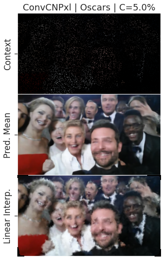
Fig. 26 Zero shot generalization of a ConvCNP trained on CelebA and evaluated on Ellen’s selfie. We also show a baseline bilinear interpolator.
From Fig. 26 we see that the model trained on single faces is able to generalise reasonably well to real world data in a zero shot fashion. One possible application of the ConvCNP is increasing the resolution of an image. This can be achieved by querying positions “in between” pixels.
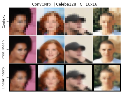
Fig. 27 Increasing the resolution of \(16 \times 16\) CelebA to \(128 \times 128\) with a ConvCNP and a baseline bilinear interpolator.
Fig. 27 demonstrates such an application. We see that the ConvCNP can indeed be used to increase the resolution of an image better than the baseline bilinear interpolator, even though it was not explicitly trained to do so!
Note
Model details, training and more plots are available in the ConvCNP Notebook. We also provide pretrained models to play around with.
Issues With the CNPF
Let’s take a step back. So far, we have seen that we can use the factorisation assumption to construct members of the CNPF, perhaps the simplest of these being the CNP. Our first observation was that while the CNP can predict simple stochatic processes, it tends to underfit when the processes are more complicated. We saw that this tendency can be addressed by adding appropriate inductive biases to the model. Specifically, the AttnCNP significantly improves upon the CNP by adding an attention mechanism to generate target-specific representations of the context set. However, both the CNP and AttnCNP fail to make meaningful predictions when data is observed outside the training range. Finally, we saw how including translation equivariance as an inductive bias led to accurate predictions that generalised elegantly to observations outside the training range.
Let’s now consider more closely the implications of the factorisation assumption, along with the Gaussian form of predictive distributions. One immediate consequence of using a Gaussian likelihood is that we cannot model multi-modal predictive distributions. To see why this might be an issue, consider making predictions for the MNIST reconstruction experiments.
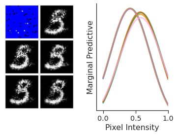
Fig. 28 Predictive distribution of a ConvCNP on an entire MNIST image (left) and marginal predictive distributions of some pixels (right).
Looking at Fig. 28, we might expect that sampling from the predictive distribution for an unobserved pixel would sometimes yield completely white values, and sometimes completely black — depending on whether the sample represents, for example, a 3 or a 5. However, a Gaussian distribution, which is unimodal (see Fig. 28 right), cannot model this multimodality.
The other major restriction is the factorisation assumption itself. First, CNPF members cannot model any dependencies in the predictive distribution over multiple target points. For example imagine that we are modelling samples from a GP. If the model is making predictions at two target locations that are “close” on the \(x\)-axis, it seems reasonable that whenever it predicts the first output to be “high”, it would predict something similar for the second, and vice versa. Yet the factorisation assumption prevents this type of correlation from occurring. Another way to view this is that the CNPF cannot produce coherent samples from its predictive distribution. In fact, sampling from the posterior corresponds to adding independent noise to the mean at each target location, resulting in samples that are discontinuous and look nothing like the underlying process:
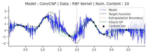
Fig. 29 Samples form the posterior predictive of a ConvCNP (Blue), and the predictive distribution of the oracle GP (Green) with RBF kernel.
Similarly, sampled images from a member of the CPNF are not coherent and look like random noise added to a picture:
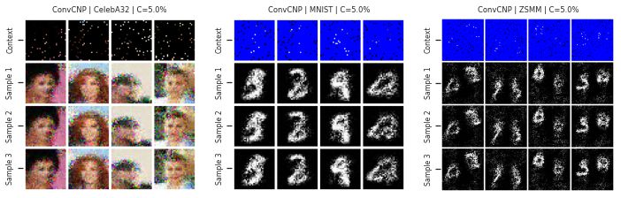
Fig. 30 Samples from the posterior predictive of an ConvCNP for CelebA, MNIST, and ZSMM.
Note\(\qquad\)Thompson Sampling
This inability to sample from the predictive may inhibit the deployment of CNPF members from several application areas for which it might otherwise be potentially well-suited. One such example is the use of Thompson sampling algorithms for e.g., contextual bandits or Bayesian optimisation, which require a model to produce samples.
In the next chapter, we will see one approach to solving both these issues by treating the representation as a latent variable. This leads us to the latent Neural Process family (LNPF).