The Neural Process Family
Deep learning has revolutionised the world of data-driven prediction, but there are still plenty of problems where it isn’t easily applicable. One such setting is the small data regime where good uncertainty estimation is required. Think, for example, of a doctor trying to predict a patient’s treatment outcome. We might have some measurements of our patient’s biophysical data since they were admitted to the hospital. However, just one patient’s data isn’t going to be enough to train a deep neural network. Furthermore, if the doctor is going to make a potentially life-changing treatment decision based on the network’s predictions, it is crucial that the network knows how certain it is, instead of being confidently wrong — something deep neural networks are prone to.
The Neural Process Family (NPF) is a collection of models (called neural processes (NPs)) that tackles both of these issues, by meta-learning a distribution over predictors, also known as a stochastic process. Meta-learning allows neural processes to incorporate data from many related tasks (e.g. many different patients in our medical example) and the stochastic process framework allows the NPF to effectively represent uncertainty.
We will unpack both the terms “meta-learning” and “stochastic process” in the following section. But before diving in, let’s consider some tasks that the NPF is particularly well-suited for.
Predicting times-series data with uncertainty. Let’s consider the task of restoring corrupted audio signals. We are given a dataset \(\mathcal{D} = \{(x^{(n)}, y^{(n)})\}_{n=1}^N\), where \(x\) are the inputs (time) and \(y\) are the outputs (sound wave amplitude), and our goal is to reconstruct the signal conditioned on \(\mathcal{D}\). If \(\mathcal{D}\) is very sparse, there could be many reasonable reconstructions — hence we should be wary of simply providing a single prediction, and instead include measures of uncertainty. Fig. 1 shows a NP being used to sample plausible interpolations of simple time-series, both periodic and non-periodic.
Fig. 1 Sample functions from the predictive distribution of ConvLNPs (the blue lines represent the predicted mean function and the shaded region shows a standard deviation on each side \([\mu-\sigma, \mu + \sigma]\)) and oracle GPs (green line represents the ground truth mean and the dashed line show a standard deviations on each side) with periodic (top) and noisy Matern kernels (bottom). Each convLNP was trained on samples from the oracle GP.
Interpolating image data with uncertainty. Imagine that we are given a satellite image of a region obscured by cloud-cover. We might need to make predictions regarding what is “behind” the occlusions. For example, the UNHCR might need to count the number of tents in a refugee camp to know how much food and healthcare supplies to send there. If clouds are obscuring a large part of the image, we might be interested not just in a single interpolation, but in the entire probability distribution over plausible interpolations. NPs can do exactly that. Fig. 2 shows a NP performing image completion with varying percentage of occluded pixels. Compared to the cubic interpolation baseline, it performs better and provides uncertainty estimates.
Fig. 2 Image completion by a ConvCNP trained on \(128 \times 128\) CelebA. The first row shows the occluded input image / context pixels. The second row shows the most probable reconstruction predicted by the NP. The third row shows the uncertainty estimates of the NP. The final row shows a baseline completion performed by cubic interpolation.
Note\(\qquad\)Outline
Our approach in this tutorial will be to walk through several prominent members of the NPF, highlighting their key advantages and drawbacks. By accompanying the exposition with code and examples, we hope to (i) make the design choices and tradeoffs associated with each model clear and intuitive, and (ii) demonstrate both the simplicity of the framework and its broad applicability.
This tutorial is split into three sections. This first page will give a broad, bird’s eye view of the entire Neural Process Family. We’ll see that the family splits naturally into two sub-families: the Conditional NPF, and the Latent NPF. These are covered in the following two pages, and there we’ll get into more detail about the different architectures in each family. In the Reproducibility section we provide the code to run all the models and generate all the plots, while the github repository contains the framework for implementing NPs.
Throughout the tutorial, we make liberal use of dropdown boxes to avoid breaking up the exposition. Feel free to skip or skim those on a first reading.
Meta Learning Stochastic Processes
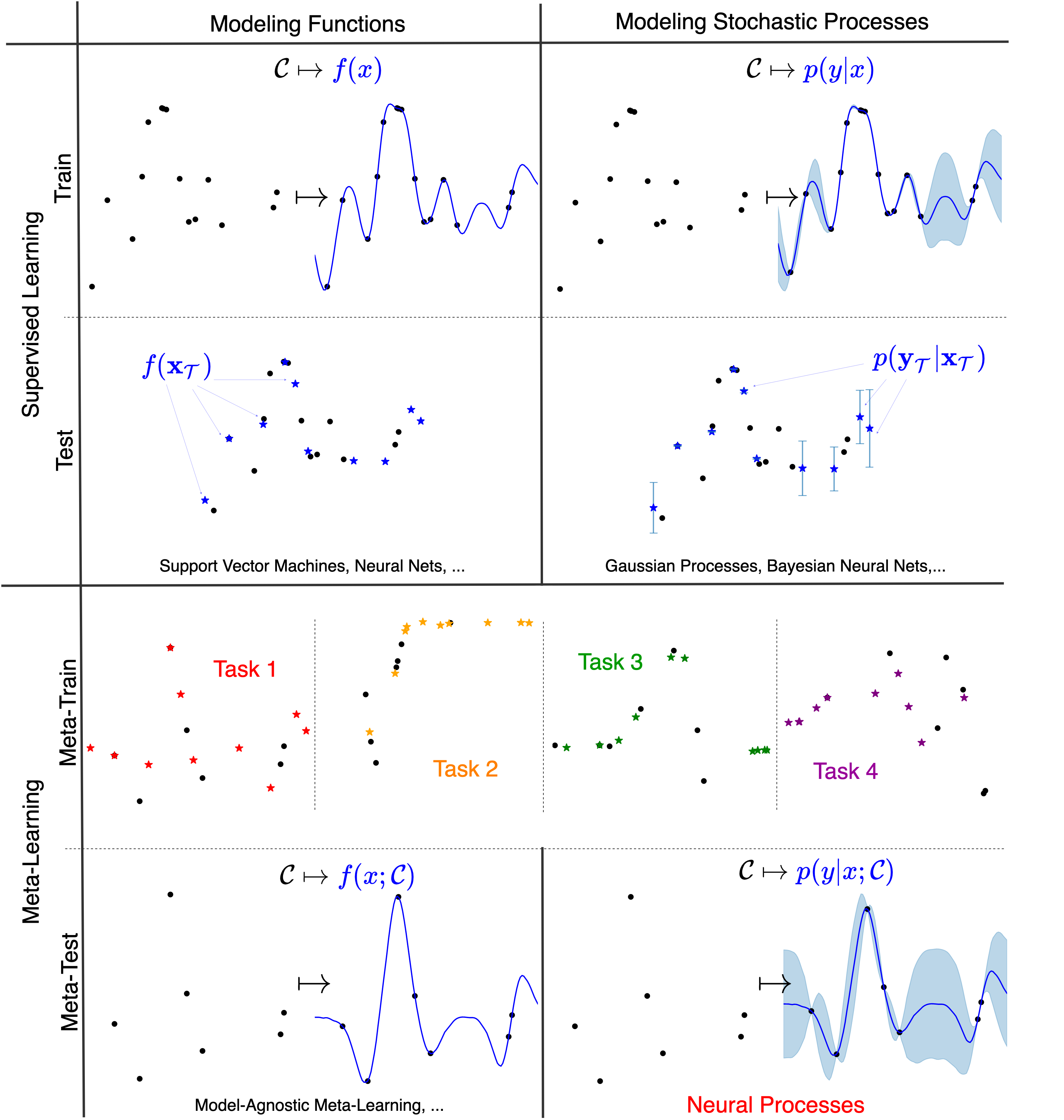
Fig. 3 Comparison between meta learning vs supervised learning, and modeling functions vs modeling stochastic processes. Neural Processes are in the lower-right quadrant. Dot are context points while stars are target points.
Meta-learning
In (deep) supervised learning, a neural network is trained to model a target function given some observations. Specifically, a network is trained on a single dataset \(\mathcal{C} := \{(x^{(c)}, y^{(c)})\}_{c=1}^C\) (which we will refer to as a context set). The trained network is then used as a predictor, \(f(x)\).
A supervised learning algorithm can thus be seen as a map that takes datasets to a predictors \(\mathcal{C} \mapsto f(x)\). At test time, a prediction at a target location \(x^{(t)}\) can be made by feeding it into the predictor to obtain \(f(x^{(t)})\). By doing so for all the test inputs (which we call target inputs) \(\mathbf{x}_{\mathcal{T}} := \{x^{(t)}\}_{t=1}^T\), we get a set of predictions \(f(\mathbf{x}_{\mathcal{T}}):= \{f(x^{(t)})\}_{t=1}^T\). The predictor is evaluated by comparing \(f(\mathbf{x}_{\mathcal{T}})\) to the ground truth target outputs \(\mathbf{y}_{\mathcal{T}} := \{y^{(t)}\}_{t=1}^T\). We will refer to a context and target set together as a task \(\mathcal{D} := (\mathcal{C}, \mathbf{x}_{\mathcal{T}}, \mathbf{y}_{\mathcal{T}})\). This standard supervised learning process is visualised in the upper left quadrant of Fig. 3.
The idea of meta-learning is learning to learn, i.e., learning how to rapidly adapt to new supervised tasks. The key insight is that, as we just saw, a supervised learning algorithm is itself a function, because it maps datasets to predictors \(\mathcal{C} \mapsto f(x)\). As a result we can model this function (the initial supervised learning algorithm) using another supervised learning algorithm, hence the name meta-learning.
To train a meta-learner, we need a large collection \(\mathcal{M}= \{ \mathcal{D_i} \}_{i=1}^{N_{\mathrm{tasks}}}\) of related datasets — a meta-dataset. The result of meta-training on this meta-dataset is a supervised learning algorithm, i.e., a map \(\mathcal{C} \mapsto f(x; \mathcal{C})\). At meta-test time, we’ll adapt the predictor to a task it has never seen before by providing it a new context set \(\mathcal{C}\). In this blog we will only consider cases where the map \(\mathcal{C} \mapsto f(x; \mathcal{C})\) is parameterised by a neural network, meaning that the adaptation (meta-test time) to a new task is done with a single forward pass, without any gradient updates! The resulting predictor, \(f(x; \mathcal{C})\), uses the information obtained during meta-learning to make predictions on this new task. The whole meta-learning process is illustrated in the bottom left quadrant of Fig. 3.
Because it can share information across tasks, meta-learning is especially well-suited to situations where each task is a small dataset, as in, e.g., few-shot learning. However, if the context set is small, should we really expect to obtain a unique predictor, \(f(x; \mathcal{C})\), from it? To relate this back to our examples, if we only observe an audio signal at a few timestamps, or an image at a few pixels, can we really uniquely reconstruct the original? What we need is to express our uncertainty, and this leads us naturally to stochastic processes.
Note\(\qquad\)Summary of Terminology
\(\mathcal{C} := \{(x^{(c)}, y^{(c)})\}_{c=1}^C\) |
Context set |
|---|---|
\(\mathbf{x}_{\mathcal{T}} := \{x^{(t)}\}_{t=1}^T\) |
Target inputs |
\(\mathbf{y}_{\mathcal{T}} := \{y^{(t)}\}_{t=1}^T\) |
Target outputs |
\(\mathcal{T} := (\mathbf{x}_{\mathcal{T}}, \mathbf{y}_{\mathcal{T}}) = \{(x^{(t)}, y^{(t)})\}_{t=1}^T\) |
Target set |
\(f(\mathbf{x}_{\mathcal{T}}; \mathcal{C}) := \{f(x^{(t)}; \mathcal{C})\}_{t=1}^T\) |
Predictions |
\(\mathcal{D} := (\mathcal{C}, \mathcal{T}) = \{(x^{(n)}, y^{(n)})\}_{n=1}^{T+C}\) |
Dataset/task |
\(\mathcal{M} := \{ \mathcal{D}^{(i)} \}_{i=1}^{N_{\mathrm{tasks}}}\) |
Meta-dataset |
Stochastic Process Prediction
We’ve seen that we can think of meta-learning as learning a map directly from context sets \(\mathcal{C}\) to predictor functions \(f(x; \mathcal{C})\). However, there are many situations where a predictor \(f(x; \mathcal{C})\) that cannot estimate its uncertainty with error-bars isn’t good enough. Quantifying uncertainty is crucial for decision-making, and has many applications such as in model-based reinforcement learning, Bayesian optimisation and out-of-distribution detection.
Given target inputs \(\mathbf{x}_{\mathcal{T}}\), what we need is not a single prediction \(f(\mathbf{x}_{\mathcal{T}}; \mathcal{C})\), but rather a distribution over predictions \(p(\mathbf{y}_{\mathcal{T}}| \mathbf{x}_{\mathcal{T}}; \mathcal{C})\). As long as these distributions are consistent with each other for different choices of \(\mathbf{x}_{\mathcal{T}}\), this is actually equivalent to specifying a distribution over functions, \(f(x; \mathcal{C})\). In mathematics, this is known as a stochastic process (SP). Each predictor sampled from this distribution would represent a plausible interpolation of the data, and the diversity of the samples would reflect the uncertainty in our predictions — think back to Fig. 1. Hence, the NPF can be viewed as using neural networks to meta-learn a map from datasets to predictive stochastic processes. This is where the name Neural Process comes from, and is illustrated in the bottom right quadrant of Fig. 3.
Advanced\(\qquad\)Stochastic Process Consistency
In the previous discussion, we considered specifying a stochastic process (SP) by specifying \(p(\mathbf{y}_{\mathcal{T}} | \mathbf{x}_{\mathcal{T}}; \mathcal{C})\) for all finite collections of target inputs \(\mathbf{x}_{\mathcal{T}}\). Each distribution for a given \(\mathbf{x}_{\mathcal{T}}\) is referred to as a finite marginal of the SP. Can we stitch together all of these finite marginals to obtain a single SP? The Kolmogorov extension theorem tells us that we can, as long as the marginals are consistent with each other under permutation and marginalisation:
To illustrate these consistency conditions, let’s look at some artificial examples of finite marginals that are not consistent. Let \(x^{(1)}, x^{(2)}\) be two target inputs, with \(y^{(1)}, y^{(2)}\) the corresponding random outputs.
Consider a collection of finite marginals with \(y^{(1)} \sim \mathcal{N}(0, 1)\) and \([y^{(1)}, y^{(2)}] \sim \mathcal{N}([10, 0], \mathbf{I})\). What is the mean of \(y^{(1)}\)?
Consider a collection with \([y^{(1)}, y^{(2)}] \sim \mathcal{N}([0, 0], \mathbf{I})\) and \([y^{(2)}, y^{(1)}] \sim \mathcal{N}([1, 1], \mathbf{I})\). What is the mean of \(y^{(1)}\)? What is the mean of \(y^{(2)}\)?
We see the problem here: inconsistent marginals lead to self-contradictory predictions! In the first example, the marginals were not consistent under marginalisation: marginalising out \(y^{(2)}\) from the distribution of \([y^{(1)}, y^{(2)}]\) did not yield the distribution of \(y^{(1)}\). In the second case, the marginals were not consistent under permutation: the distributions differed depending on whether you considered \(y^{(1)}\) first or \(y^{(2)}\) first. Later we’ll prove that this problem will never occur for NPs — for a fixed context set \(\mathcal{C}\), the NPF predictive distributions \(p(y|x;\mathcal{C})\) always define a consistent stochastic process.
So far, we’ve only considered what happens when you fix the context set and vary the target inputs. There is one more kind of consistency that we might expect SP predictions to satisfy: consistency among predictions with different context sets. Consider two input-output pairs, \((x^{(1)}, y^{(1)})\) and \((x^{(2)}, y^{(2)})\). The product rule of probability tells us that the joint predictive density must satisfy
This essentially states that the distribution over \(y^{(1)}, y^{(2)}\) obtained by autoregressive sampling should be independent of the order in which the sampling is performed. Unfortunately, this is not guaranteed to be the case for NPs, i.e., it is possible that
The lack of consistency for different context sets is the reason we use the notation \(p(y|x;\mathcal{C})\) instead of \(p(y|x,\mathcal{C})\) as standard rules of probabilities cannot be used for \(\mathcal{C}\). In practice, NPs yields good predictive performance even though they can violate this consistency.
This point of view of NPs as outputting predictive stochastic processes is helpful for making theoretical statements about the NPF. It also helps us contrast the NPF with another classical machine learning method for stochastic process prediction, Gaussian processes (GPs), which do not incorporate meta-learning (illustrated in the top right quadrant of Fig. 3). In this tutorial, we use GPs mainly to benchmark the NPF and provide synthetic datasets. In contrast to GP prediction, NPs use the expressivity of deep neural networks in their mapping. In order to do this, each member of the NPF has to address these questions: 1) How can we use neural networks to parameterise a map from datasets to predictive distributions over arbitrary target sets? 2) How can we learn this map?
Note\(\qquad\)Gaussian Processes
Fig. 1 also shows the predictive mean and error-bars of the ground truth Gaussian process (GP) used to generate the data. Unlike NPs, GPs require the user to specify a kernel function to model the data. GPs are attractive due to the fact that exact prediction in GPs can be done in closed form. However, this has computational complexity \(\mathcal{O}(|\mathcal{C}|^3)\) in the dataset size, which limits the application of exact GPs for large datasets. Many accessible introductions to GPs are available online. Some prime examples are Distill’s visual exploration, Neil Lawrence’s post, or David Mackay’s video lecture.
We note that there is a close relationship between GPs and NPs. Recall that given an appropriate kernel function \(k\), \(\mathcal{C}\), and any collection of target inputs \(\mathbf{x}_{\mathcal{T}}\), a GP defines the following posterior predictive distribution:
where we denote \(K_{\mathcal{T}, \mathcal{C}}\) as the matrix constructed by evaluating the kernel at the inputs of the target set with those of the context set, and similarly for \(K_{\mathcal{C}, \mathcal{C}}\), \(K_{\mathcal{C}, \mathcal{T}}\), and \(K_{\mathcal{T}, \mathcal{T}}\). Thus, we can think of posterior inference in GPs as a map from context sets \(\mathcal{C}\) to distributions over predictive functions, just as for NPs.
In this tutorial, we mainly use GPs to specify simple synthetic stochastic processes for benchmarking. We then train NPs to perform GP prediction. Since we can obtain the exact GP predictive distribution in closed form, we can use GPs to test the efficacy of NPs. It is important to remember, however, that NPs can model a much broader range of SPs than GPs can (e.g. natural images, SPs with multimodal marginals), are more computationally efficient at test time, and can learn directly from data without the need to hand-specify a kernel.
Parameterising Neural Processes
Here we will discuss how to parametrise NPs. As a reminder, here are three design goals that we want each NP to satisfy:
Use neural networks. The map from context sets to predictive distributions should be parametrized by a neural network. We will use a subscript \(\theta\) to denote all the parameters of the network, \(p_{\theta}(\mathbf{y}_{\mathcal{T}}| \mathbf{x}_{\mathcal{T}}; \mathcal{C})\).
The context set \(\mathcal{C}\) should be treated as a set. This differs from standard vector-valued inputs in that: i) a set may have varying sizes; ii) a set has no intrinsic ordering. The second point means that NPs should be permutation invariant, i.e., \(p_{\theta}(\mathbf{y}_{\mathcal{T}}| \mathbf{x}_{\mathcal{T}}; \mathcal{C}) = p_{\theta}(\mathbf{y}_{\mathcal{T}}| \mathbf{x}_{\mathcal{T}}; \pi(\mathcal{C}))\) for any permutation operator \(\pi\).
Consistency. The resulting predictive distributions \(p_{\theta}(\mathbf{y}_{\mathcal{T}}| \mathbf{x}_{\mathcal{T}}; \mathcal{C})\) should be consistent with each other for varying \(\mathbf{x}_{\mathcal{T}}\) to ensure that NPs give rise to proper stochastic processes — see advanced dropdown above for more details.
To satisfy these requirements, NPs first map the entire context set to a representation, \(R\), using an encoder \(\mathrm{Enc}_{\theta}\). Specifically, the encoder is always going to be of form \(\mathrm{Enc}_{\theta}(\mathcal{C}) = \rho \left ( \sum_{c=1}^C \phi(x^{(c)}, y^{(c)}) \right)\) for appropriate \(\rho\) and \(\phi\), which are defined using neural networks. The sum operation in the encoder is key as it ensures permutation invariance — due to the commutativity of the sum operation — and that the resulting \(R\) “lives” in the same space regardless of the number of context points \(C\).
After that, the NPF splits into two sub-families depending on whether or not the representation is used to define a stochastic latent variable. These sub-families are called the conditional Neural Process family (CNPF), and the latent Neural Process family (LNPF):
In the CNPF, the predictive distribution at any set of target inputs \(\mathbf{x}_{\mathcal{T}}\) is factorised conditioned on \(R\). That is, \(p_{\theta}(\mathbf{y}_{\mathcal{T}} | \mathbf{x}_{\mathcal{T}}; \mathcal{C}) = \prod_{t=1}^T p_{\theta}(y^{(t)} | x^{(t)}, R)\).
In the LNPF, the encoding \(R\) is used to define a global latent variable \(\mathbf{z} \sim p_{\theta}(\mathbf{z} | R)\). The predictive distribution is then factorised conditioned on \(\mathbf{z}\). That is, \(p_{\theta}(\mathbf{y}_{\mathcal{T}} | \mathbf{x}_{\mathcal{T}}; \mathcal{C}) = \int \prod_{t=1}^T p_{\theta}(y^{(t)} | x^{(t)}, \mathbf{z}) p_{\theta}(\mathbf{z} | R) \, \mathrm{d}\mathbf{z}\).
We will call the decoder, \(\mathrm{Dec}_{\theta}\), the map parametrizing the predictive distribution using the target input \(x^{(t)}\) and the encoding of the context set — \(R\) in the case of the CNPF and (samples of) \(z\) for the LNPF. Typically the predictive distribution is Gaussian meaning that the decoder predicts a mean \(\mu^{(t)}\) and a variance \(\sigma^{2(t)}\). As we will later show, it is the factorisation assumptions in the decoder that ensure our consistency requirement.
Concrete Example
As a concrete example of what a Neural Process looks like, Fig. 4 shows a schematic animation of the forward pass of a Conditional Neural Process (CNP), the simplest member of the CNPF. We see that every \((x, y)\) pair in the context set (here with three datapoints) is passed through an Multi-Layer Perceptron (MLP) \(e\) to obtain a local encoding. The local encodings \(\{r_1, r_2, r_3\}\) are then aggregated by a mean pooling \(a\) to a representation \(r\). Finally, the representation \(r\) is fed into another MLP \(d\) along with the target input to yield the mean and variance of the predictive distribution of the target output \(y\). We’ll take a much more detailed look at the CNP later.
Fig. 4 Schematic representation of CNP forward pass taken from Marta Garnelo.
The forward pass for members of both the CNPF and LNPF is represented schematically in Fig. 5. For the LNPF there is an extra step of sampling the latent variable \(\mathbf{z}\) in between \(R\) and \(\mathrm{Dec}_{\theta}\).1
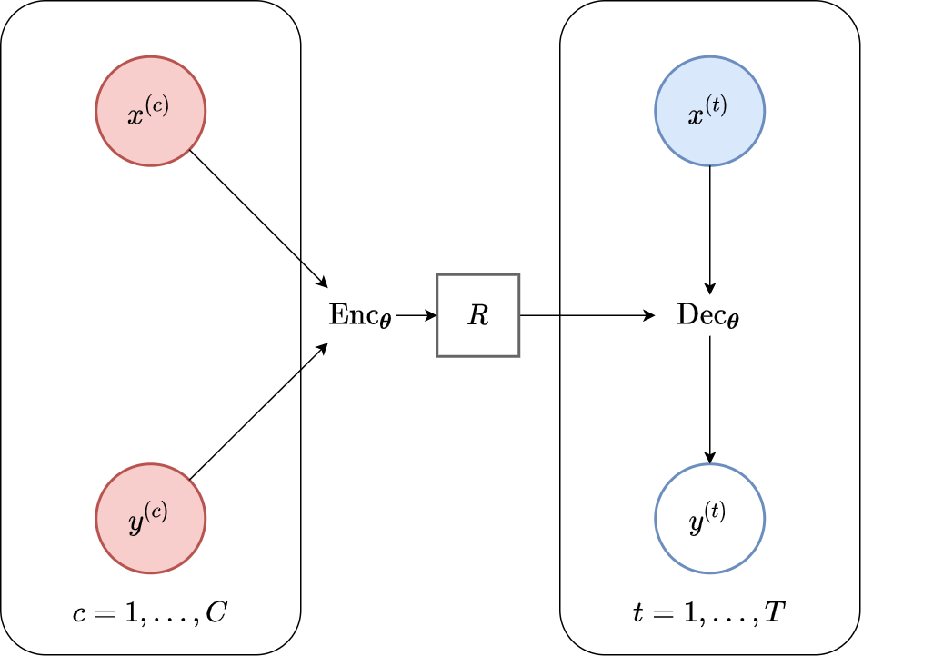
Fig. 5 High level computational graph of the Neural Process Family.
As we’ll see in the following pages of this tutorial, the CNPF and LNPF come with their own advantages and disadvantages. Roughly speaking, the LNPF allows us to model dependencies in the predictive distribution over the target set, at the cost of requiring us to approximate an intractable objective function.
Furthermore, even within each family, there are myriad choices that can be made. The most important is the choice of encoder architecture. Each of these choices will lead to neural processes with different inductive biases and capabilities. As a teaser, we provide a very brief summary of the neural processes considered in this tutorial (This should be skimmed for now, but feel free to return here to get a quick overview once each model has been introduced. Clicking on each model brings you to the Reproducibility page which includes code for running the model):
Model |
Encoder |
Spatial generalisation |
Predictive fit quality |
Additional Assumption |
|---|---|---|---|---|
MLP + Mean-pooling |
No |
Underfits |
None |
|
MLP + Attention |
No |
Less underfitting, jagged samples |
None |
|
SetConv + CNN + SetConv |
Yes |
Less underfitting, smooth samples |
Translation Equivariance |
In the CNPF and LNPF pages of this tutorial, we’ll dig into the details of how all these members of the NPF are specified in practice, and what these terms really mean. For now, we simply note the range of options and tradeoffs. To recap, we’ve (schematically!) thought about how to parameterise a map from observed context sets \(\mathcal{C}\) to predictive distributions at any target inputs \(\mathbf{x}_{\mathcal{T}}\) with neural networks. Next, we consider how to train such a map, i.e. how to learn the parameters \(\theta\).
Meta-Training in the NPF
To perform meta-learning, we require a meta-dataset or a dataset of datasets. In the meta-learning literature, each dataset in the meta-dataset is referred to as a task. For the NPF, this means having access to many independent samples of functions from the data-generating process. Each sampled function is then a task. We would like to use this meta-dataset to learn how to make predictions at a target set upon observing a context set. To do this, we use an episodic training procedure, common in meta-learning. Each episode can be summarised in five steps:
Sample a task \(\mathcal{D}\) from \(\{ \mathcal{D}_i \}_{i=1}^{N_{\mathrm{tasks}}}\).
Randomly split the task into context and target sets: \(\mathcal{D} = \mathcal{C} \cup \mathcal{T}\).
Pass \(\mathcal{C}\) through the Neural Process to obtain the predictive distribution at the target inputs, \(p_\theta(\mathbf{y}_{\mathcal{T}} | \mathbf{x}_{\mathcal{T}}; \mathcal{C})\).
Compute the log likelihood \(\mathcal{L} = \log p_\theta(\mathbf{y}_{\mathcal{T}} | \mathbf{x}_{\mathcal{T}}; \mathcal{C})\) which measures the predictive performance on the target set.8 Note that for the LNPF, we will have to compute an approximation or a lower bound of the log-likelihood objective.
Compute the gradient \(\nabla_{\theta}\mathcal{L}\) for stochastic gradient optimisation.
The episodes are repeated until training converges. Intuitively, this procedure encourages the NPF to produce predictions that fit an unseen target set, given access to only the context set. Once meta-training is complete, if the Neural Process generalises well, it will be able to do this for brand new, unseen context sets. To recap, we’ve seen how the NPF can be thought of as a family of meta-learning algorithms, taking entire datasets as input, and providing predictions with a single forward pass.
Advanced\(\qquad\)Maximum-Likelihood Training
To better understand the objective \(\mathcal{L}(\theta ; \mathcal{C}, \mathcal{T} ) = \log p_\theta(\mathbf{y}_{\mathcal{T}} | \mathbf{x}_{\mathcal{T}}; \mathcal{C})\) —which we refer to as maximum-likelihood training— let \(p(\mathcal{D}) = p(\mathcal{C}, \mathcal{T})\) be the task distribution, that is, the distribution from which we sample tasks in the episodic training procedure. Then, we can express the meta-objective as an expectation over the task distribution:
Here \(\mathrm{KL}\) is the KL-divergence, which is a measure of how different two distributions are, and \(\mathrm{const.}\) is a constant that is independent of \(\theta\). Hence we can see that maximising the meta-learning objective is equivalent to minimising the task averaged KL-divergence between the NPF predictive \(p_\theta(\mathbf{y}_{\mathcal{T}} | \mathbf{x}_{\mathcal{T}}; \mathcal{C})\) and the conditional distribution \(p(\mathbf{y}_{\mathcal{T}} | \mathbf{x}_{\mathcal{T}} , \mathcal{C})\) of the task distribution.
This point of view also helps us see the potential issues with maximum-likelihood training if \(p(\mathcal{D})\) is not truly representative of the data-generating process. For example, if all of the tasks sampled from \(p(\mathcal{D})\) have their \(x\)-values bounded in a range \([-a, a]\), then the expected KL will not include any contributions from \(p_\theta(y| x; \mathcal{C})\) when \(x\) is outside of that range. Thus there is no direct incentive for the algorithm to learn a reasonable predictive distribution for that value of \(x\). To avoid this problem, we should make our meta-dataset as representative of the tasks we expect to encounter in the future as possible.
Another way of addressing some of these issues is to bake appropriate inductive biases into the Neural Process. In the next page of this tutorial, we will see that Convolutional Neural Processes use translation equivariance to make accurate predictions for \(x\)-values outside the training range when the underlying data-generating process is stationary.
Summary of NPF Properties
Would an NPF be a good fit for your machine learning problem? To summarise, we note the advantages and disadvantages of the NPF:
✓ Fast predictions on new context sets at test time. Often, training a machine learning model on a new dataset is computationally expensive. However, meta-learning allows the NPF to incorporate information from a new context set and make predictions with a single forward pass. Typically the complexity will be linear or quadratic in the context set size instead of cubic as with standard Gaussian process regression.
✓ Well calibrated uncertainty. Often meta-learning is applied to situations where each task has only a small number of examples at test time (also known as few-shot learning). These are exactly the situations where we should have uncertainty in our predictions, since there are many possible ways to interpolate a context set with few points. The NPF learns to represent this uncertainty during episodic training.
✓ Data-driven expressivity. The enormous flexibility of deep learning architectures means that the NPF can learn to model very intricate predictive distributions directly from the data. The user mainly has to specify the inductive biases of the network architecture, e.g. convolutional vs attentive.
However, these advantages come at the cost of the following disadvantages:
✗ The need for a large dataset for meta-training. Meta-learning requires training on a large dataset of target and context points sampled from different functions, i.e., a large dataset of datasets. In some situations, a dataset of datasets may simply not be available. Furthermore, although predicting on a new context set after meta-training is fast, meta-training itself can be computationally expensive depending on the size of the network and the meta-dataset.
✗ Underfitting and smoothness issues. The NPF predictive distribution has been known to underfit the context set, and also sometimes to provide unusually jagged predictions for regression tasks. The sharpness and diversity of the image samples for the LNPF could also be improved. However, improvements are being made on this front, with both the attentive and convolutional variants of the NPF providing significant advances.
In summary, we’ve taken a bird’s eye view of the Neural Process Family and seen how they specify a map from datasets to stochastic processes, and how this map can be trained via meta-learning. We’ve also seen some of their use-cases and properties. Let’s now dive into the actual architectures! In the next two pages we’ll cover everything you need to know to get started with the models in Conditional and Latent Neural Process Families.
- 1
The general computational graph of the NPF actually has a latent variable \(\mathbf{z}\). Indeed, the CNPF may be thought of as the LNPF in the case when the latent variable \(\mathbf{z}\) is constrained to be deterministic (\(p_{\theta}(\mathbf{z} | R)\) is a Dirac delta function).
- 2
- 3
[GSR+18] — in this paper and elsewhere in the Neural Process literature, the authors refer to latent neural processes simply as neural processes. In this tutorial we use the term “neural process” to refer to both conditional neural processes and latent neural processes. We reserve the term “latent neural process” specifically for the case when there is a stochastic latent variable \(\mathbf{z}\).
- 4
[KMS+19] — this paper only introduced the latent variable Attentive LNP, but one can easily drop the latent variable to obtain the Attentive CNP.
- 5
- 6
- 7
- 8
During training the performance is usually measured on both the context and target set, i.e. we append the context set to the target set.